14 ML Serving Methods
In this article, we’ll cover:
- Criteria for choosing ML deployment types
- Key considerations when selecting ML serving methods
- Detailed insights into online real-time inference, asynchronous inference, and offline batch transform
Let’s dive in!
14.1 Criteria for Choosing ML Deployment Types
Deploying ML models effectively requires understanding four critical aspects: throughput, latency, data, and infrastructure. These factors interact closely, and trade-offs between them significantly impact your user experience and product reliability.
Throughput
Throughput refers to how many inference requests a system can handle within a specific timeframe, typically measured in requests per second (RPS). For example, consider an online retail website during a flash sale event. The system must handle a sudden influx of user requests efficiently. If, historically, the ML system processes 50 requests simultaneously in 100 milliseconds, it achieves a throughput of 500 requests per second. However, if during the sale, the volume of requests increases to 750 requests per second, then the throughput has increased by 50%.
High throughput often requires scalable infrastructure and parallel processing capabilities, whether through clusters or GPUs. And how we anticipate throughput to change in the future can impact the technology we choose in order to allow for scaling up and/or down.
Latency
Latency is the time it takes for a system to process a single inference request from when it is received until the result is returned. Latency is critical in real-time applications where quick response times are essential, such as in live user interactions, fraud detection, or any system requiring immediate feedback. For example, the average latency of OpenAI’s API is the average response time from when a user sends a request, and the service provides a result that is accessible within your application.
The latency is the sum of the network I/O, serialization and deserialization, and the LLM’s inference time. Meanwhile, the throughput is the average number of requests the API processes and serves a second. Low-latency systems require optimized and often more costly infrastructure, such as faster processors, lower network latency, and possibly edge computing to reduce the distance data needs to travel.
Throughput-Latency Tradeoff
When considering the design of your ML system, there is often a tradeoff to be made between throughput and latency. For example, a lower latency translates to higher throughput when the service processes one query simultaneously. If the service takes 100 ms to process requests, this translates to a throughput of 10 requests per second. If the latency reaches 10 ms per request, the throughput rises to 100 requests per second.
However, to complicate things, many ML systems adopt a batching strategy to simultaneously pass multiple data samples to the model. In this case, a lower latency can translate into lower throughput; in other words, a higher latency maps to a higher throughput.
For example, if you process 20 batched requests in 100 ms, the latency is 100 ms, while the throughput is 200 requests per second. If you process 60 requests in 200 ms, the latency is 200 ms, while the throughput rises to 300 requests per second. Thus, even when batching requests at serving time, it’s essential to consider the minimum latency accepted for a good user experience.
Data
The type, size, and complexity of data significantly influence throughput and latency by determining how efficiently the ML system processes requests. Structured, tabular data is typically lightweight, leading to relatively low latency and high throughput because models can quickly handle many simple computations in parallel. Conversely, complex data types like high-resolution images, videos, or lengthy text passages require more intensive computational resources, potentially increasing latency and reducing throughput.
For instance, deploying an image-recognition model that processes high-resolution images will inherently require more computing power and time per inference request, raising latency and lowering overall throughput. Similarly, Large Language Models (LLMs), which process extensive and context-rich text data, demand significant computation for each request, often necessitating specialized infrastructure (like GPUs or TPUs) to maintain acceptable performance. Therefore, it’s essential to align data characteristics with appropriate deployment strategies and infrastructure to balance performance and cost effectively.
Infrastructure
Infrastructure refers to the underlying hardware, software, networking, and system architecture that supports deploying and operating ML models. It provides essential resources for model deployment, scaling, and maintenance, encompassing computing power, memory, storage solutions, networking components, and the software stack.
- High throughput systems: For high throughput, infrastructure needs to be scalable to handle large data volumes and high request rates, typically involving parallel processing, distributed systems, and specialized hardware like high-end GPUs.
- Low latency systems: To achieve low latency, infrastructure should be optimized to reduce processing time, often necessitating faster CPUs, GPUs, specialized hardware accelerators, and potentially edge computing to minimize data travel distance. However, prioritizing low latency, particularly when batching requests, can lead to underutilized hardware capacity. Processing fewer requests per second results in idle computing resources, which raises overall processing costs. Thus, selecting infrastructure tailored to your specific latency and throughput requirements is crucial for optimizing cost and efficiency.
Designing the system’s infrastructure must also account for specific data requirements, such as choosing appropriate storage solutions for large datasets and implementing efficient retrieval methods for quick data access.
For instance, many ML systems leverage offline training for model development. Consequently, this part of the system is typically designed for high throughput, enabling the processing of large volumes of data efficiently by utilizing scalable infrastructure like GPU clusters or distributed systems. Conversely, if the inference part of the ML system leverages online inference, then infrastructure for this part of the system will be optimized primarily for low latency to ensure fast, responsive interactions, often involving dedicated hardware accelerators or edge computing to minimize delays. By tailoring system design differently for training (high throughput) and inference (low latency), you can effectively meet the distinct business needs and performance expectations of each scenario.
With this in mind, before picking a specific deployment type, you should ask yourself questions such as:
- What throughput is required, based on minimum, average, and maximum expected demand?
- How many simultaneous requests will the system need to handle (1, 10, 1k, 1 million, etc.)?
- What are the latency requirements (e.g., 1 ms, 10 ms, 1 second)?
- How will the system scale—based on CPU load, request volume, queue size, data size, or a combination?
- What are your cost constraints?
- What type and size of data will the system process (images, text, tabular data; 100 MB, 1 GB, 10 GB)?
Considering these factors thoroughly impacts your application’s user experience and reliability. A successful ML product requires not only accuracy but also responsiveness and stability. For instance, a 2016 Google study found that 53% of users abandon mobile sites taking longer than three seconds to load, highlighting latency’s significant impact on user retention.
14.2 Understanding Inference Deployment Types
Three fundamental ML deployment architectures exist for serving models:
- Online Real-time Inference
- Asynchronous Inference
- Offline Batch Transform
Each approach balances latency, throughput, and costs differently based on your application’s specific requirements. And each one can also impact how the end-user will interact with the model.
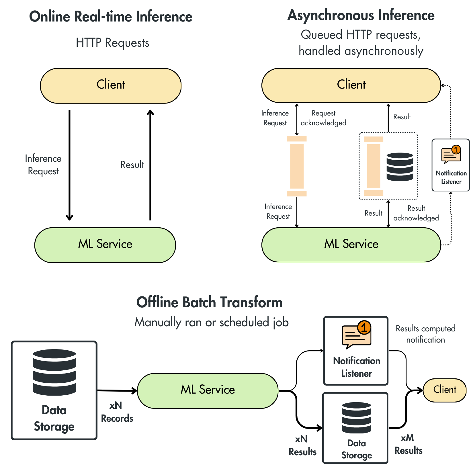
1. Online Real-time Inference
Real-time inference involves immediate, synchronous client-server interactions through HTTP requests, typically via REST APIs or gRPC.
- REST APIs are broadly accessible but slower. They typically use JSON to pass data between the client and server. This approach is usually taken when serving models outside your internal network to the broader public. For example, OpenAI’s API implements a REST API protocol.
- gRPC offers higher speed but requires more complex implementation. You have to implement protobuf schemas in your client application, which are more tedious to work with than JSON structures. The benefit, however, is that protobuf objects can be compiled into bytes, making the network transfers much faster. Thus, this protocol is often adopted for internal services within the same ML system.
Real-time inference suits applications needing immediate responses, such as interactive chatbots or recommendation systems. This deployment requires responsive, scalable infrastructure, though scaling efficiently and avoiding underutilization can be challenging.
Advantages:
- Immediate responses, suitable for interactive applications
- Simple, direct client-server communication
Drawbacks:
- Higher infrastructure costs for maintaining low latency
- Resource underutilization during low traffic
- Challenging to scale efficiently
2. Asynchronous Inference
Asynchronous inference processes requests in a queue without immediate response. This requires a robust infrastructure that queues the messages to be processed by the ML service later on. When the results are ready, you can leverage multiple techniques to send them to the client. For example, depending on the size of the result, you can put it either in a different queue or an object storage dedicated to storing the results. The client can either adopt a polling mechanism that checks on a schedule if there are new results or adopt a push strategy and implement a notification system to inform the client when the results are ready.
Advantages:
- Efficiently handles traffic spikes without immediate scaling
- Reduces infrastructure costs due to asynchronous processing
- Doesn’t block the client - the client can submit the inference request and go on doing other work while the system processes the request.
Drawbacks:
- Higher latency, unsuitable for time-sensitive tasks
Ideal for tasks like document summarization or computationally intensive processing that can tolerate some delay.
3. Offline Batch Transform
Batch transform is about processing large volumes of data simultaneously, either on a schedule or triggered manually. In a batch transform architecture, the ML service pulls data from a storage system, processes it in a single operation, and then stores the results in storage. The storage system can be implemented as an object storage like AWS S3 or a data warehouse like GCP BigQuery.
Unlike the asynchronous inference architecture, a batch transform design is optimized for high throughput with permissive latency requirements. When real-time predictions are unnecessary, this approach can significantly reduce costs, as processing data in big batches is the most economical method. Moreover, the batch transform architecture is the simplest way to serve a model, accelerating development time.
Advantages:
- High throughput, cost-effective
- Suitable for applications tolerant of delayed predictions
Drawbacks:
- Significant latency, unsuitable for real-time applications
Commonly used for daily/weekly/monthly recommendations, analytics, or periodic data processing tasks. For example, if we implement a recommender system for a video streaming application, having a delay of one day for the predicted movies and TV shows might work because you don’t consume these products at a high frequency. But suppose you make a recommender system for a social media platform. In that case, delaying one day or even one hour is unacceptable, as you constantly want to provide fresh content to the user.
Batch transform shines in scenarios where high throughput is needed, like data analytics or periodic reporting. However, it’s unsuitable for real-time applications due to its high latency and requires careful planning and scheduling to manage large datasets effectively. That’s why it is an offline serving method.
14.3 Conclusion
Effectively deploying ML models involves balancing throughput, latency, data characteristics, and infrastructure. Understanding these trade-offs and selecting the appropriate deployment architecture ensures optimal performance, user satisfaction, and cost efficiency.