8 Lesson 3a: Linear Regression
Linear regression, a staple of classical statistical modeling, is one of the simplest algorithms for doing supervised learning. Though it may seem somewhat dull compared to some of the more modern statistical learning approaches described in later modules, linear regression is still a useful and widely applied statistical learning method. Moreover, it serves as a good starting point for more advanced approaches; as we will see in later modules, many of the more sophisticated statistical learning approaches can be seen as generalizations to or extensions of ordinary linear regression. Consequently, it is important to have a good understanding of linear regression before studying more complex learning methods. This module introduces linear regression with an emphasis on prediction, rather than inference. An excellent and comprehensive overview of linear regression is provided in Kutner et al. (2005). See Faraway (2016) for a discussion of linear regression in R.
8.2 Prerequisites
This lesson leverages the following packages:
# Helper packages
library(dplyr)    # for data manipulation
library(ggplot2)  # for awesome graphics

# Modeling packages
library(tidymodels)

# Model interpretability packages
library(vip)      # variable importance
We’ll also continue working with the ames data set:
# stratified sampling with the rsample package
ames <- AmesHousing::make_ames()

set.seed(123)
split  <- initial_split(ames, prop = 0.7, strata = "Sale_Price")
ames_train  <- training(split)
ames_test   <- testing(split)
8.3 Simple linear regression
Pearson’s correlation coefficient is often used to quantify the strength of the linear association between two continuous variables. In this section, we seek to fully characterize that linear relationship. Simple linear regression (SLR) assumes that the statistical relationship between two continuous variables (say \(X\) and \(Y\)) is (at least approximately) linear:
\[\begin{equation} Y_i = \beta_0 + \beta_1 X_i + \epsilon_i, \quad \text{for } i = 1, 2, \dots, n, \end{equation}\]
where \(Y_i\) represents the i-th response value, \(X_i\) represents the i-th feature value, \(\beta_0\) and \(\beta_1\) are fixed, but unknown constants (commonly referred to as coefficients or parameters) that represent the intercept and slope of the regression line, respectively, and \(\epsilon_i\) represents noise or random error. In this module, we’ll assume that the errors are normally distributed with mean zero and constant variance \(\sigma^2\), denoted \(\stackrel{iid}{\sim} \left(0, \sigma^2\right)\). Since the random errors are centered around zero (i.e., \(E\left(\epsilon\right) = 0\)), linear regression is really a problem of estimating a conditional mean:
\[\begin{equation} E\left(Y_i | X_i\right) = \beta_0 + \beta_1 X_i. \end{equation}\]
For brevity, we often drop the conditional piece and write \(E\left(Y | X\right) = E\left(Y\right)\). Consequently, the interpretation of the coefficients is in terms of the average, or mean response. For example, the intercept \(\beta_0\) represents the average response value when \(X = 0\) (it is often not meaningful or of interest and is sometimes referred to as a bias term). The slope \(\beta_1\) represents the increase in the average response per one-unit increase in \(X\) (i.e., it is a rate of change).
8.4 Estimation
Ideally, we want estimates of \(\beta_0\) and \(\beta_1\) that give us the “best fitting” line. But what is meant by “best fitting”? The most common approach is to use the method of least squares (LS) estimation; this form of linear regression is often referred to as ordinary least squares (OLS) regression. There are multiple ways to measure “best fitting”, but the LS criterion finds the “best fitting” line by minimizing the residual sum of squares (RSS):
\[\begin{equation} RSS\left(\beta_0, \beta_1\right) = \sum_{i=1}^n\left[Y_i - \left(\beta_0 + \beta_1 X_i\right)\right]^2 = \sum_{i=1}^n\left(Y_i - \beta_0 - \beta_1 X_i\right)^2. \end{equation}\]
The LS estimates of \(\beta_0\) and \(\beta_1\) are denoted as \(\widehat{\beta}_0\) and \(\widehat{\beta}_1\), respectively. Once obtained, we can generate predicted values, say at \(X = X_{new}\), using the estimated regression equation:
\[\begin{equation} \widehat{Y}_{new} = \widehat{\beta}_0 + \widehat{\beta}_1 X_{new}, \end{equation}\]
where \(\widehat{Y}_{new} = \widehat{E\left(Y_{new} | X = X_{new}\right)}\) is the estimated mean response at \(X = X_{new}\).
With the Ames housing data, suppose we wanted to model a linear relationship between the total above ground living space of a home (Gr_Liv_Area) and sale price (Sale_Price). To perform an OLS regression model in R we can use the linear_reg() model object, which by default will use the lm engine:
model1 <- linear_reg() %>%
   fit(Sale_Price ~ Gr_Liv_Area, data = ames_train)
The fitted model (model1) is displayed in the left plot below where the points represent the values of Sale_Price in the training data. In the right plot, the vertical lines represent the individual errors, called residuals, associated with each observation. The OLS criterion identifies the “best fitting” line that minimizes the sum of squares of these residuals.
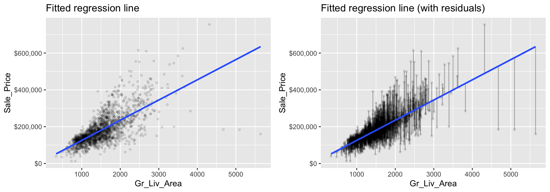
Figure 8.1: The least squares fit from regressing sale price on living space for the the Ames housing data. Left: Fitted regression line. Right: Fitted regression line with vertical grey bars representing the residuals.
We can extract our fitted model results with tidy():
tidy(model1)
## # A tibble: 2 × 5
##   term        estimate std.error statistic   p.value
##   <chr>          <dbl>     <dbl>     <dbl>     <dbl>
## 1 (Intercept)   15938.   3852.        4.14 3.65e-  5
## 2 Gr_Liv_Area     110.      2.42     45.3  5.17e-311
The estimated coefficients from our model are \(\widehat{\beta}_0 =\) 15938.17 and \(\widehat{\beta}_1 =\) 109.67. To interpret, we estimate that the mean selling price increases by 109.67 for each additional one square foot of above ground living space. This simple description of the relationship between the sale price and square footage using a single number (i.e., the slope) is what makes linear regression such an intuitive and popular modeling tool.
One drawback of the LS procedure in linear regression is that it only provides estimates of the coefficients; it does not provide an estimate of the error variance \(\sigma^2\)! LS also makes no assumptions about the random errors. These assumptions are important for inference and in estimating the error variance which we’re assuming is a constant value \(\sigma^2\). One way to estimate \(\sigma^2\) (which is required for characterizing the variability of our fitted model), is to use the method of maximum likelihood (ML) estimation (see Kutner et al. (2005) Section 1.7 for details). The ML procedure requires that we assume a particular distribution for the random errors. Most often, we assume the errors to be normally distributed. In practice, under the usual assumptions stated above, an unbiased estimate of the error variance is given as the sum of the squared residuals divided by \(n - p\) (where \(p\) is the number of regression coefficients or parameters in the model):
\[\begin{equation} \widehat{\sigma}^2 = \frac{1}{n - p}\sum_{i = 1} ^ n r_i ^ 2, \end{equation}\]
where \(r_i = \left(Y_i - \widehat{Y}_i\right)\) is referred to as the \(i\)th residual (i.e., the difference between the \(i\)th observed and predicted response value). The quantity \(\widehat{\sigma}^2\) is also referred to as the mean square error (MSE) and its square root is denoted RMSE (see here for discussion on these metrics).
Typically, these error metrics are computed on a separate validation set or using cross-validation; however, they can also be computed on the same training data the model was trained on as illustrated here.
In R, the RMSE of a linear model, along with many other model metrics, can be extracted with glance(). sigma in the results below is the RMSE value, which is 56787.94. This means that, on average, our model’s predicted values are $56787.94 off from the actual price! Not very impressive.
# RMSE
glance(model1)
## # A tibble: 1 × 12
## r.squared adj.r.…¹ sigma stati…² p.value df logLik AIC BIC devia…³ df.re…⁴
## <dbl> <dbl> <dbl> <dbl> <dbl> <dbl> <dbl> <dbl> <dbl> <dbl> <int>
## 1 0.501 0.500 56788. 2052. 5.17e-311 1 -25337. 50680. 50697. 6.60e12 2047
## # … with 1 more variable: nobs <int>, and abbreviated variable names ¹adj.r.squared,
## # ²statistic, ³deviance, ⁴df.residual
## # ℹ Use `colnames()` to see all variable names
# We can compute the MSE by simply squaring RMSE (sigma)
glance(model1) %>%
mutate(MSE = sigma^2) %>%
select(sigma, MSE, everything())
## # A tibble: 1 × 13
## sigma MSE r.squ…¹ adj.r…² stati…³ p.value df logLik AIC BIC devia…⁴
## <dbl> <dbl> <dbl> <dbl> <dbl> <dbl> <dbl> <dbl> <dbl> <dbl> <dbl>
## 1 56788. 3.22e9 0.501 0.500 2052. 5.17e-311 1 -25337. 50680. 50697. 6.60e12
## # … with 2 more variables: df.residual <int>, nobs <int>, and abbreviated variable names
## # ¹r.squared, ²adj.r.squared, ³statistic, ⁴deviance
## # ℹ Use `colnames()` to see all variable names8.5 Inference
How accurate are the LS of \(\beta_0\) and \(\beta_1\)? Point estimates by themselves are not very useful. It is often desirable to associate some measure of an estimates variability. The variability of an estimate is often measured by its standard error (SE)—the square root of its variance. If we assume that the errors in the linear regression model are \(\stackrel{iid}{\sim} \left(0, \sigma^2\right)\), then simple expressions for the SEs of the estimated coefficients exist and are displayed in the column labeled std.error in the output from tidy(). From this, we can also derive simple \(t\)-tests to understand if the individual coefficients are statistically significant from zero. The t-statistics for such a test are nothing more than the estimated coefficients divided by their corresponding estimated standard errors (i.e., in the output from tidy(), t value (aka statistic) = estimate / std.error). The reported t-statistics measure the number of standard deviations each coefficient is away from 0. Thus, large t-statistics (greater than two in absolute value, say) roughly indicate statistical significance at the \(\alpha = 0.05\) level. The p-values for these tests are also reported by tidy() in the column labeled p.value.
Under the same assumptions, we can also derive confidence intervals for the coefficients. The formula for the traditional \(100\left(1 - \alpha\right)\)% confidence interval for \(\beta_j\) is
\[\begin{equation} \widehat{\beta}_j \pm t_{1 - \alpha / 2, n - p} \widehat{SE}\left(\widehat{\beta}_j\right). \end{equation}\]
In R, we can construct such (one-at-a-time) confidence intervals for each coefficient using confint() on the model1$fit object. For example, a 95% confidence intervals for the coefficients in our SLR example can be computed using
confint(model1$fit, level = 0.95)
##                2.5 %     97.5 %
## (Intercept) 8384.213 23492.1336
## Gr_Liv_Area  104.920   114.4149
To interpret, we estimate with 95% confidence that the mean selling price increases between 104.92 and 114.41 for each additional one square foot of above ground living space. We can also conclude that the slope \(\beta_1\) is significantly different from zero (or any other pre-specified value not included in the interval) at the \(\alpha = 0.05\) level. This is also supported by the output from tidy().
Most statistical software, including R, will include estimated standard errors, t-statistics, etc. as part of its regression output. However, it is important to remember that such quantities depend on three major assumptions of the linear regression model:
- Independent observations
- The random errors have mean zero, and constant variance
- The random errors are normally distributed
If any or all of these assumptions are violated, then remedial measures need to be taken. For instance, weighted least squares (and other procedures) can be used when the constant variance assumption is violated. Transformations (of both the response and features) can also help to correct departures from these assumptions. The residuals are extremely useful in helping to identify how parametric models depart from such assumptions.
8.6 Multiple linear regression
In practice, we often have more than one predictor. For example, with the Ames housing data, we may wish to understand if above ground square footage (Gr_Liv_Area) and the year the house was built (Year_Built) are (linearly) related to sale price (Sale_Price). We can extend the SLR model so that it can directly accommodate multiple predictors; this is referred to as the multiple linear regression (MLR) model. With two predictors, the MLR model becomes:
\[\begin{equation} Y = \beta_0 + \beta_1 X_1 + \beta_2 X_2 + \epsilon, \end{equation}\]
where \(X_1\) and \(X_2\) are features of interest. In our Ames housing example, \(X_1\) represents Gr_Liv_Area and \(X_2\) represents Year_Built.
In R, multiple linear regression models can be fit by separating all the features of interest with a +:
model2 <- linear_reg() %>%
   fit(Sale_Price ~ Gr_Liv_Area + Year_Built, data = ames_train)

tidy(model2)
## # A tibble: 3 × 5
##   term          estimate std.error statistic   p.value
##   <chr>            <dbl>     <dbl>     <dbl>     <dbl>
## 1 (Intercept) -2102905.   69441.       -30.3 9.17e-167
## 2 Gr_Liv_Area       93.8      2.07      45.3 1.17e-310
## 3 Year_Built      1087.      35.6       30.5 3.78e-169
The LS estimates of the regression coefficients are \(\widehat{\beta}_1 =\) 93.828 and \(\widehat{\beta}_2 =\) 1086.852 (the estimated intercept is -2.1029046^{6}. In other words, every one square foot increase to above ground square footage is associated with an additional $93.83 in mean selling price when holding the year the house was built constant. Likewise, for every year newer a home is there is approximately an increase of $1,086.85 in selling price when holding the above ground square footage constant.
Now, instead of modeling sale price with the the “best fitting” line that minimizes residuals, we are modeling sale price with the best fitting hyperplane that minimizes the residuals, which is illustrated below.
Figure 8.2: Average home sales price as a function of year built and total square footage.
You may notice that the fitted plane in the above image is flat; there is no curvature. This is true for all linear models that include only main effects (i.e., terms involving only a single predictor). One way to model curvature is to include interaction effects. An interaction occurs when the effect of one predictor on the response depends on the values of other predictors. In linear regression, interactions can be captured via products of features (i.e., \(X_1 \times X_2\)). A model with two main effects can also include a two-way interaction. For example, to include an interaction between \(X_1 =\) Gr_Liv_Area and \(X_2 =\) Year_Built, we introduce an additional product term:
\[\begin{equation} Y = \beta_0 + \beta_1 X_1 + \beta_2 X_2 + \beta_3 X_1 X_2 + \epsilon. \end{equation}\]
Note that in R, we use the : operator to include an interaction (technically, we could use * as well, but x1 * x2 is shorthand for x1 + x2 + x1:x2 so is slightly redundant):
interaction_model <- linear_reg() %>%
   fit(Sale_Price ~ Gr_Liv_Area + Year_Built + Gr_Liv_Area:Year_Built, data = ames_train)

tidy(interaction_model)
## # A tibble: 4 × 5
##   term                      estimate   std.error statistic  p.value
##   <chr>                        <dbl>       <dbl>     <dbl>    <dbl>
## 1 (Intercept)            -810498.    210537.         -3.85 1.22e- 4
## 2 Gr_Liv_Area               -729.       127.         -5.75 1.01e- 8
## 3 Year_Built                 431.       107.          4.03 5.83e- 5
## 4 Gr_Liv_Area:Year_Built       0.417      0.0642      6.49 1.04e-10
The curvature that interactions capture can be illustrated in the contour plot below. The left plot illustrates a regression model with main effects only. Note how the fitted regression surface is flat (i.e., it does not twist or bend). While the fitted regression surface with interaction is displayed in the right side plot and you can see the curvature of the relationship induced.
Interaction effects are quite prevalent in predictive modeling. Since linear models are an example of parametric modeling, it is up to the analyst to decide if and when to include interaction effects. In later chapters, we’ll discuss algorithms that can automatically detect and incorporate interaction effects (albeit in different ways). It is also important to understand a concept called the hierarchy principle—which demands that all lower-order terms corresponding to an interaction be retained in the model—when considering interaction effects in linear regression models.
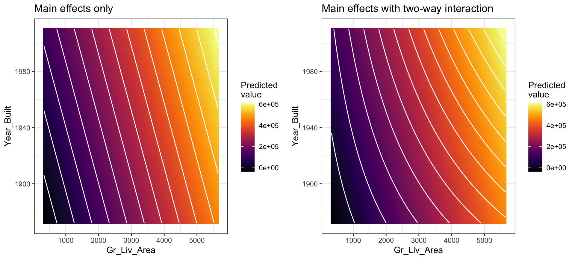
Figure 8.3: In a three-dimensional setting, with two predictors and one response, the least squares regression line becomes a plane. The ‘best-fit’ plane minimizes the sum of squared errors between the actual sales price (individual dots) and the predicted sales price (plane).
In general, we can include as many predictors as we want, as long as we have more rows than parameters! The general multiple linear regression model with p distinct predictors is
\[\begin{equation} Y = \beta_0 + \beta_1 X_1 + \beta_2 X_2 + \cdots + \beta_p X_p + \epsilon, \end{equation}\]
where \(X_i\) for \(i = 1, 2, \dots, p\) are the predictors of interest. Note some of these may represent interactions (e.g., \(X_3 = X_1 \times X_2\)) between or transformations3 (e.g., \(X_4 = \sqrt{X_1}\)) of the original features. Unfortunately, visualizing beyond three dimensions is not practical as our best-fit plane becomes a hyperplane. However, the motivation remains the same where the best-fit hyperplane is identified by minimizing the RSS. The code below creates a third model where we use all features in our data set as main effects (i.e., no interaction terms) to predict Sale_Price.
# include all possible main effects
model3 <- linear_reg() %>%
fit(Sale_Price ~ ., data = ames_train)
# print estimated coefficients in a tidy data frame
tidy(model3)
## # A tibble: 300 × 5
## term estimate std.error stati…¹ p.value
## <chr> <dbl> <dbl> <dbl> <dbl>
## 1 (Intercept) -27256503. 11016450. -2.47 0.0134
## 2 MS_SubClassOne_Story_1945_and_Older 3901. 3575. 1.09 0.275
## 3 MS_SubClassOne_Story_with_Finished_Attic_All_Ages -5389. 12164. -0.443 0.658
## 4 MS_SubClassOne_and_Half_Story_Unfinished_All_Ages -441. 13942. -0.0316 0.975
## 5 MS_SubClassOne_and_Half_Story_Finished_All_Ages 1037. 7250. 0.143 0.886
## 6 MS_SubClassTwo_Story_1946_and_Newer -6669. 5510. -1.21 0.226
## 7 MS_SubClassTwo_Story_1945_and_Older 1574. 6074. 0.259 0.795
## 8 MS_SubClassTwo_and_Half_Story_All_Ages 3408. 10149. 0.336 0.737
## 9 MS_SubClassSplit_or_Multilevel -6670. 11673. -0.571 0.568
## 10 MS_SubClassSplit_Foyer 1492. 7512. 0.199 0.843
## # … with 290 more rows, and abbreviated variable name ¹statistic
## # ℹ Use `print(n = ...)` to see more rows8.7 Assessing model accuracy
We’ve fit three main effects models to the Ames housing data: a single predictor, two predictors, and all possible predictors. But the question remains, which model is “best”? To answer this question we have to define what we mean by “best”. In our case, we’ll use the RMSE metric and cross-validation to determine the “best” model.
In essence, we are going to train our three different models using k-fold cross validation. The model that has the lowest average cross validation RMSE is considered the model that generalizes to new data the best.
First, we’ll perform 10-fold cross validation on the single predictor model (Sales_Price ~ Gr_Liv_Area):
# create our 10-fold cross validation object
set.seed(8451)
kfolds <- vfold_cv(ames_train, v = 10)

# create our linear regression model object
lm_mod <- linear_reg()

# add model object and our formula spec to a workflow object
lm_wflow <- workflow() %>%
   add_model(lm_mod) %>%
   add_formula(Sale_Price ~ Gr_Liv_Area)

# fit our model across the 10-fold CV
lm_fit_cv <- lm_wflow %>%
   fit_resamples(kfolds)

# assess results
results <- collect_metrics(lm_fit_cv)
results
## # A tibble: 2 × 6
##   .metric .estimator      mean     n   std_err .config
##   <chr>   <chr>          <dbl> <int>     <dbl> <chr>
## 1 rmse    standard   56358.       10 2854.     Preprocessor1_Model1
## 2 rsq     standard       0.516    10    0.0296 Preprocessor1_Model1
The resulting cross-validated RMSE is $56,358.36 (this is the average RMSE across the 10 CV folds). How should we interpret this? When applied to unseen data, the predictions this model makes are, on average, about $56,358.36 off from the actual sale price.
We can perform cross-validation on the other two models in a similar fashion, which we do in the code chunk below.
# two predictor variables
workflow() %>%
   add_model(lm_mod) %>%
   add_formula(Sale_Price ~ Gr_Liv_Area + Year_Built) %>%
   fit_resamples(kfolds) %>%
   collect_metrics()
## # A tibble: 2 × 6
##   .metric .estimator      mean     n   std_err .config
##   <chr>   <chr>          <dbl> <int>     <dbl> <chr>
## 1 rmse    standard   46634.       10 2692.     Preprocessor1_Model1
## 2 rsq     standard       0.667    10    0.0259 Preprocessor1_Model1

# using all available predictor variables
workflow() %>%
   add_model(lm_mod) %>%
   add_formula(Sale_Price ~ .) %>%
   fit_resamples(kfolds) %>%
   collect_metrics()
## # A tibble: 2 × 6
##   .metric .estimator      mean     n   std_err .config
##   <chr>   <chr>          <dbl> <int>     <dbl> <chr>
## 1 rmse    standard   39318.       10 7429.     Preprocessor1_Model1
## 2 rsq     standard       0.786    10    0.0584 Preprocessor1_Model1
Extracting the results for each model, we see that by adding more information via more predictors, we are able to improve the out-of-sample cross validation performance metrics. Specifically, our cross-validated RMSE reduces from $46,634 (the model with two predictors) down to $39,318 (for our full model). In this case, the model with all possible main effects performs the “best” (compared with the other two).
Now, this process of comparing multiple models is fairly common. And when we look at the code above we see a similar process - basically we want to train a linear regression using k-fold resampling across three different formula specifications (1 predictor, 2 predictors, and all available predictors).
Rather than re-use the same workflow code we can:
- Create three different model specifications (aka recipes)
- Combine these different recipes along with the model(s) of interest into a workflow set object.
We could pass multiple models to train across each formula but here we are only interested in training a linear regression model (
linear_reg()) on each formula specification.
# create three different model recipes
one_pred <- recipe(Sale_Price ~ Gr_Liv_Area, data = ames_train)
two_pred <- recipe(Sale_Price ~ Gr_Liv_Area + Year_Built, data = ames_train)
all_pred <- recipe(Sale_Price ~ ., data = ames_train) %>%
   step_other(all_nominal_predictors(), threshold = 0.05)

# combine into a list
model_specs <- list(
   model1 = one_pred,
   model2 = two_pred,
   model3 = all_pred
   )

lm_models <- workflow_set(model_specs, list(lm = linear_reg()), cross = FALSE)
lm_models
## # A workflow set/tibble: 3 × 4
##   wflow_id  info             option    result
##   <chr>     <list>           <list>    <list>
## 1 model1_lm <tibble [1 × 4]> <opts[0]> <list [0]>
## 2 model2_lm <tibble [1 × 4]> <opts[0]> <list [0]>
## 3 model3_lm <tibble [1 × 4]> <opts[0]> <list [0]>
Next, we’d like to train our models using k-fold cross validation – or in essence, fit these models using resampling. To do so, we will use a purrr-like function called workflow_map(). This function takes an initial argument of the function to apply (fit_resamples() to the workflows, followed by options to that function (i.e. kfolds).
Basically we are using workflow_map() like a
for loop or map function to iterate over each
formula specification and perform some task -
fit_resamples() in this example.
lm_results <- lm_models %>%
workflow_map("fit_resamples", resamples = kfolds)
collect_metrics(lm_results) %>%
filter(.metric == "rmse")
## # A tibble: 3 × 9
## wflow_id .config preproc model .metric .estim…¹ mean n std_err
## <chr> <chr> <chr> <chr> <chr> <chr> <dbl> <int> <dbl>
## 1 model1_lm Preprocessor1_Model1 recipe linear_reg rmse standard 56358. 10 2854.
## 2 model2_lm Preprocessor1_Model1 recipe linear_reg rmse standard 46634. 10 2692.
## 3 model3_lm Preprocessor1_Model1 recipe linear_reg rmse standard 32878. 10 3717.
## # … with abbreviated variable name ¹.estimatorAs we add more model comparisons it can be helpful to visualize the results, which we can do with autoplot(). Here we just see that model3 has the highest RMSE value compared to model2 and model1.
This isn’t the most informative plot right now but as we get into other models and start tuning hyperparameters we’ll see how this plot becomes more useful.
autoplot(lm_results)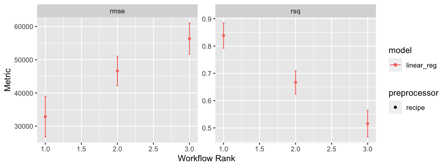
8.8 Feature importance
Ok, so we found a linear regression model that performs best compared to other linear regression models. Our next goal is often to interpret the model structure. Linear regression models provide a very intuitive model structure as they assume a monotonic linear relationship between the predictor variables and the response. The linear relationship part of that statement just means, for a given predictor variable, it assumes for every one unit change in a given predictor variable there is a constant change in the response. As discussed earlier in the lesson, this constant rate of change is provided by the coefficient for a predictor. The monotonic relationship means that a given predictor variable will always have a positive or negative relationship. But how do we determine the most influential variables?
Variable importance seeks to identify those variables that are most influential in our model. For linear regression models, this is most often measured by the absolute value of the t-statistic for each model parameter used. Rather than search through each of the
We can use vip::vip() to extract and plot the most important variables. The importance measure is normalized from 100 (most important) to 0 (least important). The plot below illustrates that the top 5 most important variables are Second_Flr_SF, First_Flr_SF, Kitchen_QualTypical, KitchenQualGood, and Mist_Val respectively.
# extract best performing model and
# train it on the train/test split
# and extract the final fit model
best_lm_model <- lm_results %>%
   extract_workflow(id = 'model3_lm') %>%
   last_fit(split) %>%
   extract_fit_parsnip()

# plot top 10 influential features
best_lm_model %>%
   vip(num_features = 20)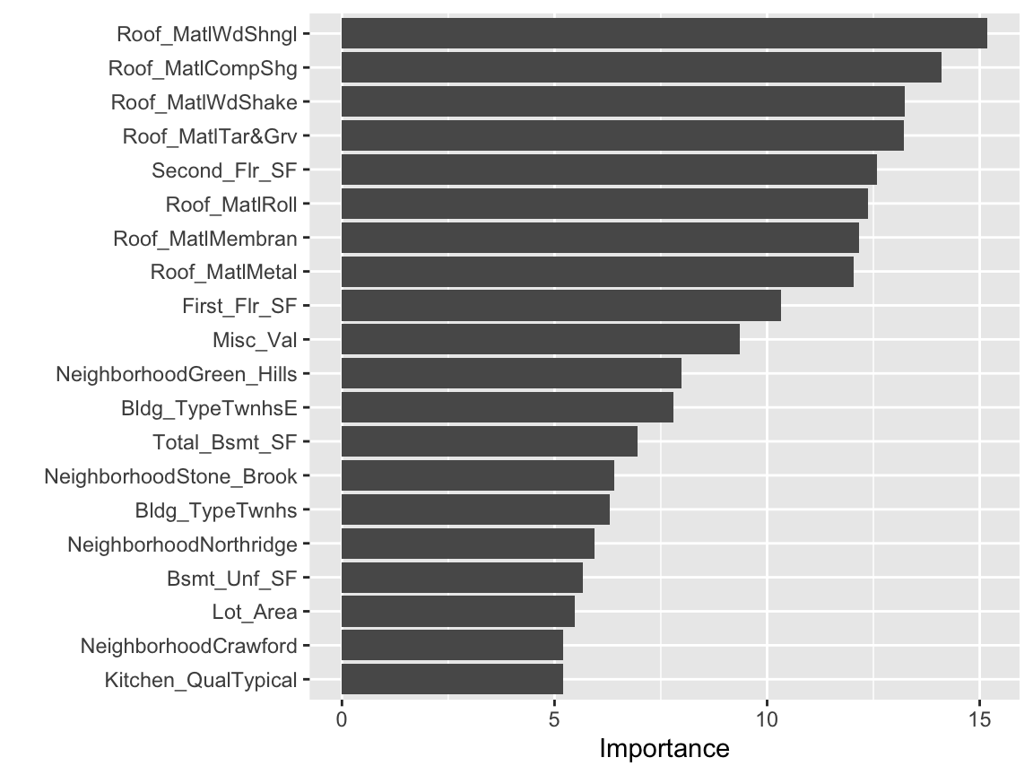
This is basically saying that our model finds that these are the most influential features in our data set that have the largest impact on the predicted outcome. If we order our data based on the t-statistic we see similar results.
tidy(best_lm_model) %>%
   arrange(desc(statistic))
## # A tibble: 150 × 5
##    term                           estimate std.error statistic  p.value
##    <chr>                             <dbl>     <dbl>     <dbl>    <dbl>
##  1 Second_Flr_SF                      68.0      5.10     13.3  8.92e-39
##  2 First_Flr_SF                       50.5      4.72     10.7  6.06e-26
##  3 NeighborhoodNorthridge_Heights  26604.    4738.        5.62 2.25e- 8
##  4 Overall_Qualother               25476.    4553.        5.60 2.51e- 8
##  5 Latitude                       283889.   55373.        5.13 3.25e- 7
##  6 Overall_QualVery_Good           21118.    4169.        5.07 4.46e- 7
##  7 Bsmt_ExposureGd                 15429.    3049.        5.06 4.59e- 7
##  8 Sale_ConditionNormal            14155.    2825.        5.01 5.95e- 7
##  9 Screen_Porch                       58.7     12.5       4.68 3.10e- 6
## 10 Mas_Vnr_Area                       25.4      5.75      4.42 1.05e- 5
## # … with 140 more rows
## # ℹ Use `print(n = ...)` to see more rows
We can also use these results above to see the impact that these features have on the predicted value. For example, for every one additional unit of Second_Flr_SF our model adds $67.98 to the predicted Sale_Price.
8.9 Final thoughts
Linear regression is usually the first supervised learning algorithm you will learn. The approach provides a solid fundamental understanding of the supervised learning task; however, as we’ll discuss in the next lesson there are several concerns that result from the assumptions required by linear regression. Future lessons will demonstrate extensions of linear regression that integrate dimension reduction steps into the algorithm that help address some of the problems with linear regression, and we’ll see how more advanced supervised algorithms can provide greater flexibility and improved accuracy. Nonetheless, understanding linear regression provides a foundation that will serve you well in learning these more advanced methods.
8.10 Exercises
Using the Boston housing data set where the response feature is the
median value of homes within a census tract (cmedv):
-
Pick a single feature and apply a simple linear regression model.
- Interpret the feature’s coefficient
- What is the model’s performance?
-
Pick another feature to add to the model.
- Before applying the model why do you think this feature will help?
- Apply a linear regression model with the two features and compare to the simple linear model.
- Interpret the coefficients.
-
Now apply a model that includes all the predictors.
- How does this model compare to the previous two?
-
Compare the above three models using 10-fold cross validation.
- Which model do you think will generalize to unseen data the best?
- Using the best model from this resampling procedure, identify the top 3 most influential features for this model and interpret their coefficients.