10 Manipulating Data

“During the course of doing data analysis and modeling, a significant amount of time is spent on data preparation: loading, cleaning, transforming, and rearranging. Such tasks are often reported to take up 80% or more of an analyst’s time.” — Wes McKinney, creator of Pandas, in Python for Data Analysis

In our previous chapter, we explored how to access, index, and subset data from a pandas DataFrame. These are essential skills for understanding and navigating real-world datasets. Now we take the next step: learning how to manipulate data.

As a data analyst or scientist, you will spend much of your time transforming raw data into something clean, interpretable, and analysis-ready. This chapter provides the foundation for doing just that. You’ll learn to rename columns, create new variables, deal with missing values, and apply functions to your data — all of which are fundamental skills in the data science workflow.

By the end of this chapter, you will be able to:

Rename and reformat column names
Perform arithmetic operations on columns
Add, drop, and overwrite columns in a DataFrame
Handle missing values using identification and imputation techniques
Apply custom functions to DataFrame columns using .apply() and .map()

📓 Follow Along in Colab!

As you read through this chapter, we encourage you to follow along using the companion notebook in Google Colab (or other editor of choice). This interactive notebook lets you run code examples covered in the chapter—and experiment with your own ideas.

👉 Open the Manipulating Data Notebook in Colab.

The Ames Housing Data

You first encountered the Ames Housing dataset back in Chapter 7, where you were challenged with the task of analyzing raw data for the Ames, Iowa housing market. In this chapter, we’ll return to the Ames data as our primary example to learn how to manipulate and prepare real-world data for analysis.

Before diving into the new concepts, take a few minutes to reacquaint yourself with the data:

How many observations are included?
What variables (columns) are present, and what kinds of information do they represent?
Can you spot any potential issues — such as inconsistent naming, unclear variable descriptions, or missing values — that might need to be addressed?

Let’s begin by loading the dataset and inspecting the first few rows:

import pandas as pd

ames = pd.read_csv('../data/ames_raw.csv')
ames.head()

	Order	PID	MS SubClass	MS Zoning	Lot Frontage	Lot Area	Street	Alley	Lot Shape	Land Contour	...	Pool QC	Fence	Misc Feature	Misc Val	Mo Sold	Yr Sold	Sale Type	Sale Condition	SalePrice
0	1	526301100	20	RL	141.0	31770	Pave	NaN	IR1	Lvl	...	NaN	NaN	NaN	0	5	2010	WD	Normal	215000
1	2	526350040	20	RH	80.0	11622	Pave	NaN	Reg	Lvl	...	NaN	MnPrv	NaN	0	6	2010	WD	Normal	105000
2	3	526351010	20	RL	81.0	14267	Pave	NaN	IR1	Lvl	...	NaN	NaN	Gar2	12500	6	2010	WD	Normal	172000
3	4	526353030	20	RL	93.0	11160	Pave	NaN	Reg	Lvl	...	NaN	NaN	NaN	0	4	2010	WD	Normal	244000
4	5	527105010	60	RL	74.0	13830	Pave	NaN	IR1	Lvl	...	NaN	MnPrv	NaN	0	3	2010	WD	Normal	189900

5 rows × 82 columns

We’ll use this dataset throughout the chapter to demonstrate how to rename columns, compute new variables, handle missing data, and apply transformations — all crucial steps in cleaning and preparing data for analysis and modeling.

10.1 Renaming Columns

One of the first things you’ll often do when working with a new dataset is clean up the column names. Column names might contain spaces, inconsistent capitalization, or other formatting quirks that make them harder to work with in code. In this section, we’ll walk through a few ways to rename columns in a DataFrame using the Ames Housing dataset.

Let’s start by looking at the current column names:

ames.columns

Index(['Order', 'PID', 'MS SubClass', 'MS Zoning', 'Lot Frontage', 'Lot Area',
       'Street', 'Alley', 'Lot Shape', 'Land Contour', 'Utilities',
       'Lot Config', 'Land Slope', 'Neighborhood', 'Condition 1',
       'Condition 2', 'Bldg Type', 'House Style', 'Overall Qual',
       'Overall Cond', 'Year Built', 'Year Remod/Add', 'Roof Style',
       'Roof Matl', 'Exterior 1st', 'Exterior 2nd', 'Mas Vnr Type',
       'Mas Vnr Area', 'Exter Qual', 'Exter Cond', 'Foundation', 'Bsmt Qual',
       'Bsmt Cond', 'Bsmt Exposure', 'BsmtFin Type 1', 'BsmtFin SF 1',
       'BsmtFin Type 2', 'BsmtFin SF 2', 'Bsmt Unf SF', 'Total Bsmt SF',
       'Heating', 'Heating QC', 'Central Air', 'Electrical', '1st Flr SF',
       '2nd Flr SF', 'Low Qual Fin SF', 'Gr Liv Area', 'Bsmt Full Bath',
       'Bsmt Half Bath', 'Full Bath', 'Half Bath', 'Bedroom AbvGr',
       'Kitchen AbvGr', 'Kitchen Qual', 'TotRms AbvGrd', 'Functional',
       'Fireplaces', 'Fireplace Qu', 'Garage Type', 'Garage Yr Blt',
       'Garage Finish', 'Garage Cars', 'Garage Area', 'Garage Qual',
       'Garage Cond', 'Paved Drive', 'Wood Deck SF', 'Open Porch SF',
       'Enclosed Porch', '3Ssn Porch', 'Screen Porch', 'Pool Area', 'Pool QC',
       'Fence', 'Misc Feature', 'Misc Val', 'Mo Sold', 'Yr Sold', 'Sale Type',
       'Sale Condition', 'SalePrice'],
      dtype='object')

You might notice that some of these column names contain spaces or uppercase letters, such as "MS SubClass" and "MS Zoning". These formatting issues can be inconvenient when writing code — especially if you’re trying to access a column using dot notation (e.g., df.column_name) or when using string methods.

Renaming Specific Columns

We can rename one or more columns using the .rename() method. This method accepts a dictionary where the keys are the original column names and the values are the new names you’d like to assign.

ames.rename(columns={'MS SubClass': 'ms_subclass', 'MS Zoning': 'ms_zoning'})

	Order	PID	ms_subclass	ms_zoning	Lot Frontage	Lot Area	Street	Alley	Lot Shape	Land Contour	...	Pool Area	Pool QC	Fence	Misc Feature	Misc Val	Mo Sold	Yr Sold	Sale Type	Sale Condition	SalePrice
0	1	526301100	20	RL	141.0	31770	Pave	NaN	IR1	Lvl	...	0	NaN	NaN	NaN	0	5	2010	WD	Normal	215000
1	2	526350040	20	RH	80.0	11622	Pave	NaN	Reg	Lvl	...	0	NaN	MnPrv	NaN	0	6	2010	WD	Normal	105000
2	3	526351010	20	RL	81.0	14267	Pave	NaN	IR1	Lvl	...	0	NaN	NaN	Gar2	12500	6	2010	WD	Normal	172000
3	4	526353030	20	RL	93.0	11160	Pave	NaN	Reg	Lvl	...	0	NaN	NaN	NaN	0	4	2010	WD	Normal	244000
4	5	527105010	60	RL	74.0	13830	Pave	NaN	IR1	Lvl	...	0	NaN	MnPrv	NaN	0	3	2010	WD	Normal	189900
...	...	...	...	...	...	...	...	...	...	...	...	...	...	...	...	...	...	...	...	...	...
2925	2926	923275080	80	RL	37.0	7937	Pave	NaN	IR1	Lvl	...	0	NaN	GdPrv	NaN	0	3	2006	WD	Normal	142500
2926	2927	923276100	20	RL	NaN	8885	Pave	NaN	IR1	Low	...	0	NaN	MnPrv	NaN	0	6	2006	WD	Normal	131000
2927	2928	923400125	85	RL	62.0	10441	Pave	NaN	Reg	Lvl	...	0	NaN	MnPrv	Shed	700	7	2006	WD	Normal	132000
2928	2929	924100070	20	RL	77.0	10010	Pave	NaN	Reg	Lvl	...	0	NaN	NaN	NaN	0	4	2006	WD	Normal	170000
2929	2930	924151050	60	RL	74.0	9627	Pave	NaN	Reg	Lvl	...	0	NaN	NaN	NaN	0	11	2006	WD	Normal	188000

2930 rows × 82 columns

This command runs without error; and if we check out our data (below) nothing seems different. Why?

ames.head(3)

	Order	PID	MS SubClass	MS Zoning	Lot Frontage	Lot Area	Street	Alley	Lot Shape	Land Contour	...	Pool QC	Fence	Misc Feature	Misc Val	Mo Sold	Yr Sold	Sale Type	Sale Condition	SalePrice
0	1	526301100	20	RL	141.0	31770	Pave	NaN	IR1	Lvl	...	NaN	NaN	NaN	0	5	2010	WD	Normal	215000
1	2	526350040	20	RH	80.0	11622	Pave	NaN	Reg	Lvl	...	NaN	MnPrv	NaN	0	6	2010	WD	Normal	105000
2	3	526351010	20	RL	81.0	14267	Pave	NaN	IR1	Lvl	...	NaN	NaN	Gar2	12500	6	2010	WD	Normal	172000

3 rows × 82 columns

That’s because .rename() returns a new DataFrame with the updated names, but it does not modify the original DataFrame unless you explicitly tell it to.

There are two common ways to make these changes permanent:

Use the inplace=True argument
Reassign the modified DataFrame to the same variable

The Pandas development team recommends the second approach (reassigning) for most use cases, as it leads to clearer and more predictable code.

ames = ames.rename(columns={'MS SubClass': 'ms_subclass', 'MS Zoning': 'ms_zoning'})
ames.head()

	Order	PID	ms_subclass	ms_zoning	Lot Frontage	Lot Area	Street	Alley	Lot Shape	Land Contour	...	Pool QC	Fence	Misc Feature	Misc Val	Mo Sold	Yr Sold	Sale Type	Sale Condition	SalePrice
0	1	526301100	20	RL	141.0	31770	Pave	NaN	IR1	Lvl	...	NaN	NaN	NaN	0	5	2010	WD	Normal	215000
1	2	526350040	20	RH	80.0	11622	Pave	NaN	Reg	Lvl	...	NaN	MnPrv	NaN	0	6	2010	WD	Normal	105000
2	3	526351010	20	RL	81.0	14267	Pave	NaN	IR1	Lvl	...	NaN	NaN	Gar2	12500	6	2010	WD	Normal	172000
3	4	526353030	20	RL	93.0	11160	Pave	NaN	Reg	Lvl	...	NaN	NaN	NaN	0	4	2010	WD	Normal	244000
4	5	527105010	60	RL	74.0	13830	Pave	NaN	IR1	Lvl	...	NaN	MnPrv	NaN	0	3	2010	WD	Normal	189900

5 rows × 82 columns

Always include columns= when using .rename(). If you don’t, Pandas will assume you are renaming index values instead of column names — and it won’t raise a warning or error if you make this mistake.

Renaming Many Columns at Once

Using .rename() works well for renaming one or two columns. But if you want to rename many columns — such as applying a consistent format across the entire DataFrame — it’s more efficient to use the .columns attribute and vectorized string methods.

Pandas provides powerful tools for working with strings through the .str accessor. For example, we can convert all column names to lowercase like this:

ames.columns.str.lower()

Index(['order', 'pid', 'ms_subclass', 'ms_zoning', 'lot frontage', 'lot area',
       'street', 'alley', 'lot shape', 'land contour', 'utilities',
       'lot config', 'land slope', 'neighborhood', 'condition 1',
       'condition 2', 'bldg type', 'house style', 'overall qual',
       'overall cond', 'year built', 'year remod/add', 'roof style',
       'roof matl', 'exterior 1st', 'exterior 2nd', 'mas vnr type',
       'mas vnr area', 'exter qual', 'exter cond', 'foundation', 'bsmt qual',
       'bsmt cond', 'bsmt exposure', 'bsmtfin type 1', 'bsmtfin sf 1',
       'bsmtfin type 2', 'bsmtfin sf 2', 'bsmt unf sf', 'total bsmt sf',
       'heating', 'heating qc', 'central air', 'electrical', '1st flr sf',
       '2nd flr sf', 'low qual fin sf', 'gr liv area', 'bsmt full bath',
       'bsmt half bath', 'full bath', 'half bath', 'bedroom abvgr',
       'kitchen abvgr', 'kitchen qual', 'totrms abvgrd', 'functional',
       'fireplaces', 'fireplace qu', 'garage type', 'garage yr blt',
       'garage finish', 'garage cars', 'garage area', 'garage qual',
       'garage cond', 'paved drive', 'wood deck sf', 'open porch sf',
       'enclosed porch', '3ssn porch', 'screen porch', 'pool area', 'pool qc',
       'fence', 'misc feature', 'misc val', 'mo sold', 'yr sold', 'sale type',
       'sale condition', 'saleprice'],
      dtype='object')

Or, we can chain multiple string methods together to standardize our column names — converting them to lowercase and replacing all spaces with underscores:

ames.columns = ames.columns.str.lower().str.replace(" ", "_")
ames.head()

	order	pid	ms_subclass	ms_zoning	lot_frontage	lot_area	street	alley	lot_shape	land_contour	...	pool_qc	fence	misc_feature	misc_val	mo_sold	yr_sold	sale_type	sale_condition	saleprice
0	1	526301100	20	RL	141.0	31770	Pave	NaN	IR1	Lvl	...	NaN	NaN	NaN	0	5	2010	WD	Normal	215000
1	2	526350040	20	RH	80.0	11622	Pave	NaN	Reg	Lvl	...	NaN	MnPrv	NaN	0	6	2010	WD	Normal	105000
2	3	526351010	20	RL	81.0	14267	Pave	NaN	IR1	Lvl	...	NaN	NaN	Gar2	12500	6	2010	WD	Normal	172000
3	4	526353030	20	RL	93.0	11160	Pave	NaN	Reg	Lvl	...	NaN	NaN	NaN	0	4	2010	WD	Normal	244000
4	5	527105010	60	RL	74.0	13830	Pave	NaN	IR1	Lvl	...	NaN	MnPrv	NaN	0	3	2010	WD	Normal	189900

5 rows × 82 columns

This makes your column names easier to type, more consistent, and less prone to errors in your code.

You can explore other string operations that work with .str by checking out the Pandas string methods documentation.

Knowledge Check

Try This!

Let’s practice cleaning up messy column names using the techniques from this section. Below is a small example dataset with inconsistent column names:

import pandas as pd

data = pd.DataFrame({
    'First Name': ['Alice', 'Bob', 'Charlie'],
    'Last-Name': ['Smith', 'Jones', 'Brown'],
    'AGE ': [25, 30, 22],
    'Email Address': ['alice@example.com', 'bob@example.com', 'charlie@example.com']
})

Your task:

Print the current column names. What formatting issues do you see?
Clean the column names by doing the following:
- Convert all column names to lowercase
- Replace any spaces or hyphens with underscores
- Strip any leading or trailing whitespace
Assign the cleaned column names back to the DataFrame.
Print the updated column names and confirm the changes.

Hint: .columns.str.lower(), .str.replace(), and .str.strip() will come in handy here!

10.2 Performing Calculations with Columns

Once your data is loaded and your columns are cleaned up, the next common task is to perform calculations on your data. This might include creating new variables, transforming existing values, or applying arithmetic operations across columns.

Let’s begin by focusing on the saleprice column in the Ames Housing dataset. This column records the sale price of each home in dollars. For example:

sale_price = ames['saleprice']
sale_price

0       215000
1       105000
2       172000
3       244000
4       189900
         ...  
2925    142500
2926    131000
2927    132000
2928    170000
2929    188000
Name: saleprice, Length: 2930, dtype: int64

These numbers are fairly large — often six digits long. In many analyses or visualizations, it can be helpful to express values in thousands of dollars instead of raw dollar amounts.

To convert the sale price to thousands, we simply divide each value by 1,000:

sale_price_k = sale_price / 1000
sale_price_k

0       215.0
1       105.0
2       172.0
3       244.0
4       189.9
        ...  
2925    142.5
2926    131.0
2927    132.0
2928    170.0
2929    188.0
Name: saleprice, Length: 2930, dtype: float64

This results in a new Series where each home’s price is now shown in thousands. For instance, a home that originally sold for $215,000 is now shown as 215.0.

At this point, sale_price_k is a new object that exists separately from the ames DataFrame. In the next section, we’ll learn how to add this new variable as a column in our DataFrame so we can use it in further analysis.

10.3 Adding and Removing Columns

Once you’ve created a new variable — like sale_price_k in the previous section — you’ll often want to add it to your existing DataFrame so it becomes part of the dataset you’re working with.

Adding Columns

In pandas, you can add a new column to a DataFrame using assignment syntax:

# example syntax
df['new_column_name'] = new_column_series

Let’s add the sale_price_k series (which represents sale prices in thousands) to the ames DataFrame:

ames['sale_price_k'] = sale_price_k
ames.head()

	order	pid	ms_subclass	ms_zoning	lot_frontage	lot_area	street	alley	lot_shape	land_contour	...	pool_qc	fence	misc_feature	misc_val	mo_sold	yr_sold	sale_type	sale_condition	saleprice	sale_price_k
0	1	526301100	20	RL	141.0	31770	Pave	NaN	IR1	Lvl	...	NaN	NaN	NaN	0	5	2010	WD	Normal	215000	215.0
1	2	526350040	20	RH	80.0	11622	Pave	NaN	Reg	Lvl	...	NaN	MnPrv	NaN	0	6	2010	WD	Normal	105000	105.0
2	3	526351010	20	RL	81.0	14267	Pave	NaN	IR1	Lvl	...	NaN	NaN	Gar2	12500	6	2010	WD	Normal	172000	172.0
3	4	526353030	20	RL	93.0	11160	Pave	NaN	Reg	Lvl	...	NaN	NaN	NaN	0	4	2010	WD	Normal	244000	244.0
4	5	527105010	60	RL	74.0	13830	Pave	NaN	IR1	Lvl	...	NaN	MnPrv	NaN	0	3	2010	WD	Normal	189900	189.9

5 rows × 83 columns

Now, you’ll see that a new column called "sale_price_k" appears at the end of the DataFrame.

Notice how the column name ('sale_price_k') is placed in quotes inside the brackets on the left-hand side, while the Series providing the data goes on the right-hand side without quotes or brackets.

This entire process can be done in a single step, without creating an intermediate variable:

ames['sale_price_k'] = ames['saleprice'] / 1000

This kind of operation is common in data science. What we’re doing here is applying vectorized math — performing arithmetic between a Series (a vector of values) and a scalar (a single constant value).

Here are a few more examples:

# Subtracting a scalar from a Series
(ames['saleprice'] - 12).head()

0    214988
1    104988
2    171988
3    243988
4    189888
Name: saleprice, dtype: int64

# Multiplying a Series by a scalar
(ames['saleprice'] * 10).head()

0    2150000
1    1050000
2    1720000
3    2440000
4    1899000
Name: saleprice, dtype: int64

# Raising a Series to a power
(ames['saleprice'] ** 2).head()

0    46225000000
1    11025000000
2    29584000000
3    59536000000
4    36062010000
Name: saleprice, dtype: int64

Vectorized operations like these are fast, efficient, and more readable than writing explicit loops.

Removing Columns

Just as easily as we can add columns, we can also remove them. This is helpful when a column is no longer needed or was created only temporarily.

To drop one or more columns from a DataFrame, use the .drop() method with the columns= argument:

ames = ames.drop(columns=['order', 'sale_price_k'])
ames.head()

	pid	ms_subclass	ms_zoning	lot_frontage	lot_area	street	alley	lot_shape	land_contour	utilities	...	pool_qc	fence	misc_feature	misc_val	mo_sold	yr_sold	sale_type	sale_condition	saleprice
0	526301100	20	RL	141.0	31770	Pave	NaN	IR1	Lvl	AllPub	...	NaN	NaN	NaN	0	5	2010	WD	Normal	215000
1	526350040	20	RH	80.0	11622	Pave	NaN	Reg	Lvl	AllPub	...	NaN	MnPrv	NaN	0	6	2010	WD	Normal	105000
2	526351010	20	RL	81.0	14267	Pave	NaN	IR1	Lvl	AllPub	...	NaN	NaN	Gar2	12500	6	2010	WD	Normal	172000
3	526353030	20	RL	93.0	11160	Pave	NaN	Reg	Lvl	AllPub	...	NaN	NaN	NaN	0	4	2010	WD	Normal	244000
4	527105010	60	RL	74.0	13830	Pave	NaN	IR1	Lvl	AllPub	...	NaN	MnPrv	NaN	0	3	2010	WD	Normal	189900

5 rows × 81 columns

This removes the "order" and "sale_price_k" columns from the DataFrame. Remember that most pandas methods return a new DataFrame by default, so you’ll need to reassign the result back to ames (or another variable) to make the change permanent.

Knowledge check

Create a utility_space variable

Create a new column utility_space that is 1/5 of the above ground living space (gr_liv_area).
You will get fractional output with step #1. See if you can figure out how to round this output to the nearest integer.
Now remove this column from your DataFrame

10.4 Overwriting columns

What if we discovered a systematic error in our data? Perhaps we find out that the “lot_area” column is not entirely accurate because the recording process includes an extra 50 square feet for every property. We could create a new column, “real_lot_area” but we’re not going to need the original “lot_area” column, and leaving it could cause confusion for others looking at our data.

A better solution would be to replace the original column with the new, recalculated, values. We can do so using the same syntax as for creating a new column.

# Subtract 50 from lot area, and then overwrite the original data.
ames['lot_area'] = ames['lot_area'] - 50
ames.head()

	pid	ms_subclass	ms_zoning	lot_frontage	lot_area	street	alley	lot_shape	land_contour	utilities	...	pool_qc	fence	misc_feature	misc_val	mo_sold	yr_sold	sale_type	sale_condition	saleprice
0	526301100	20	RL	141.0	31720	Pave	NaN	IR1	Lvl	AllPub	...	NaN	NaN	NaN	0	5	2010	WD	Normal	215000
1	526350040	20	RH	80.0	11572	Pave	NaN	Reg	Lvl	AllPub	...	NaN	MnPrv	NaN	0	6	2010	WD	Normal	105000
2	526351010	20	RL	81.0	14217	Pave	NaN	IR1	Lvl	AllPub	...	NaN	NaN	Gar2	12500	6	2010	WD	Normal	172000
3	526353030	20	RL	93.0	11110	Pave	NaN	Reg	Lvl	AllPub	...	NaN	NaN	NaN	0	4	2010	WD	Normal	244000
4	527105010	60	RL	74.0	13780	Pave	NaN	IR1	Lvl	AllPub	...	NaN	MnPrv	NaN	0	3	2010	WD	Normal	189900

5 rows × 81 columns

10.5 Calculating with Multiple Columns

Up to this point, we’ve focused on performing calculations between a column (Series) and a scalar — for example, dividing every value in saleprice by 1,000. But pandas also allows you to perform operations between columns — this is known as vector-vector arithmetic.

Let’s look at an example where we calculate a new metric: price per square foot. We can compute this by dividing the sale price of each home by its above-ground living area (gr_liv_area):

price_per_sqft = ames['saleprice'] / ames['gr_liv_area']
price_per_sqft.head()

0    129.830918
1    117.187500
2    129.420617
3    115.639810
4    116.574586
dtype: float64

Now that we’ve computed the new values, let’s add them to our DataFrame as a new column:

ames['price_per_sqft'] = price_per_sqft
ames.head()

	pid	ms_subclass	ms_zoning	lot_frontage	lot_area	street	alley	lot_shape	land_contour	utilities	...	pool_qc	fence	misc_feature	misc_val	mo_sold	yr_sold	sale_type	sale_condition	saleprice	price_per_sqft
0	526301100	20	RL	141.0	31720	Pave	NaN	IR1	Lvl	AllPub	...	NaN	NaN	NaN	0	5	2010	WD	Normal	215000	129.830918
1	526350040	20	RH	80.0	11572	Pave	NaN	Reg	Lvl	AllPub	...	NaN	MnPrv	NaN	0	6	2010	WD	Normal	105000	117.187500
2	526351010	20	RL	81.0	14217	Pave	NaN	IR1	Lvl	AllPub	...	NaN	NaN	Gar2	12500	6	2010	WD	Normal	172000	129.420617
3	526353030	20	RL	93.0	11110	Pave	NaN	Reg	Lvl	AllPub	...	NaN	NaN	NaN	0	4	2010	WD	Normal	244000	115.639810
4	527105010	60	RL	74.0	13780	Pave	NaN	IR1	Lvl	AllPub	...	NaN	MnPrv	NaN	0	3	2010	WD	Normal	189900	116.574586

5 rows × 82 columns

As before, you could write this as a one-liner:

ames['price_per_sqft'] = ames['saleprice'] / ames['gr_liv_area']

Combining Multiple Operations

You can also combine multiple columns and scalars in more complex expressions. For example, the following line combines three columns and a constant:

ames['nonsense'] = (ames['yr_sold'] + 12) * ames['gr_liv_area'] + ames['lot_area'] - 50
ames.head()

	pid	ms_subclass	ms_zoning	lot_frontage	lot_area	street	alley	lot_shape	land_contour	utilities	...	fence	misc_feature	misc_val	mo_sold	yr_sold	sale_type	sale_condition	saleprice	price_per_sqft	nonsense
0	526301100	20	RL	141.0	31720	Pave	NaN	IR1	Lvl	AllPub	...	NaN	NaN	0	5	2010	WD	Normal	215000	129.830918	3380102
1	526350040	20	RH	80.0	11572	Pave	NaN	Reg	Lvl	AllPub	...	MnPrv	NaN	0	6	2010	WD	Normal	105000	117.187500	1823234
2	526351010	20	RL	81.0	14217	Pave	NaN	IR1	Lvl	AllPub	...	NaN	Gar2	12500	6	2010	WD	Normal	172000	129.420617	2701405
3	526353030	20	RL	93.0	11110	Pave	NaN	Reg	Lvl	AllPub	...	NaN	NaN	0	4	2010	WD	Normal	244000	115.639810	4277480
4	527105010	60	RL	74.0	13780	Pave	NaN	IR1	Lvl	AllPub	...	MnPrv	NaN	0	3	2010	WD	Normal	189900	116.574586	3307568

5 rows × 83 columns

This creates a column called "nonsense" using a mix of vector-vector and vector-scalar operations. While this particular example isn’t meaningful analytically, it shows how you can chain together multiple operations in a single expression.

In practice, you’ll often calculate new variables using a combination of existing columns — for example, calculating cost efficiency, total square footage, or ratios between two quantities. Being comfortable with these kinds of operations is essential for building features and preparing data for analysis or modeling.

Knowledge check

Create a price_per_total_sqft variable

Create a new column price_per_total_sqft that is saleprice divided by the sum of gr_liv_area, total_bsmt_sf, wood_deck_sf, open_porch_sf.

10.6 Working with String Columns

So far, we’ve focused on numeric calculations — things like dividing, multiplying, and creating new variables based on numbers. But many datasets also contain non-numeric values, such as names, categories, or descriptive labels.

In pandas, string data is stored as object or string type columns, and you can perform operations on them just like you would with numbers. This is especially useful for cleaning, formatting, or combining text.

String Concatenation

A common operation with string data is concatenation — combining multiple strings together. For example, suppose we want to create a descriptive sentence using the neighborhood and sale condition of each home in the Ames dataset:

'Home in ' + ames['neighborhood'] + ' neighborhood sold under ' + ames['sale_condition'] + ' condition'

0       Home in NAmes neighborhood sold under Normal c...
1       Home in NAmes neighborhood sold under Normal c...
2       Home in NAmes neighborhood sold under Normal c...
3       Home in NAmes neighborhood sold under Normal c...
4       Home in Gilbert neighborhood sold under Normal...
                              ...                        
2925    Home in Mitchel neighborhood sold under Normal...
2926    Home in Mitchel neighborhood sold under Normal...
2927    Home in Mitchel neighborhood sold under Normal...
2928    Home in Mitchel neighborhood sold under Normal...
2929    Home in Mitchel neighborhood sold under Normal...
Length: 2930, dtype: object

This works just like string addition in Python. Each piece of text is combined row by row across the DataFrame to generate a new sentence for each observation.

String Methods with `.str`

For more advanced string operations, pandas provides a powerful set of tools through the .str accessor. This gives you access to many string-specific methods like .lower(), .replace(), .len(), and more.

Here are a few examples:

# Count the number of characters in each neighborhood name
ames['neighborhood'].str.len()

0       5
1       5
2       5
3       5
4       7
       ..
2925    7
2926    7
2927    7
2928    7
2929    7
Name: neighborhood, Length: 2930, dtype: int64

# Standardize the format of garage type labels
ames['garage_type'].str.lower().str.replace('tchd', 'tached')

0       attached
1       attached
2       attached
3       attached
4       attached
          ...   
2925    detached
2926    attached
2927         NaN
2928    attached
2929    attached
Name: garage_type, Length: 2930, dtype: object

These methods are especially helpful when cleaning messy or inconsistent text data — for example, fixing capitalization, removing whitespace, or replacing substrings.

In this chapter, we’ve only scratched the surface of working with non-numeric data. In later chapters, we’ll take a deeper look at how to clean, transform, and analyze string values, as well as how to work with date and time data — including parsing timestamps, extracting components like month and day, and calculating time differences.

For now, if you want to dig into working with string columns some more, it’s worth exploring the official Pandas documentation on string methods to see the full range of capabilities.

Whether you’re formatting text for a report, cleaning up inconsistent labels, or preparing inputs for machine learning models, working with string columns is a valuable part of your data wrangling skill set.

ames

	pid	ms_subclass	ms_zoning	lot_frontage	lot_area	street	alley	lot_shape	land_contour	utilities	...	fence	misc_feature	misc_val	mo_sold	yr_sold	sale_type	sale_condition	saleprice	price_per_sqft	nonsense
0	526301100	20	RL	141.0	31720	Pave	NaN	IR1	Lvl	AllPub	...	NaN	NaN	0	5	2010	WD	Normal	215000	129.830918	3380102
1	526350040	20	RH	80.0	11572	Pave	NaN	Reg	Lvl	AllPub	...	MnPrv	NaN	0	6	2010	WD	Normal	105000	117.187500	1823234
2	526351010	20	RL	81.0	14217	Pave	NaN	IR1	Lvl	AllPub	...	NaN	Gar2	12500	6	2010	WD	Normal	172000	129.420617	2701405
3	526353030	20	RL	93.0	11110	Pave	NaN	Reg	Lvl	AllPub	...	NaN	NaN	0	4	2010	WD	Normal	244000	115.639810	4277480
4	527105010	60	RL	74.0	13780	Pave	NaN	IR1	Lvl	AllPub	...	MnPrv	NaN	0	3	2010	WD	Normal	189900	116.574586	3307568
...	...	...	...	...	...	...	...	...	...	...	...	...	...	...	...	...	...	...	...	...	...
2925	923275080	80	RL	37.0	7887	Pave	NaN	IR1	Lvl	AllPub	...	GdPrv	NaN	0	3	2006	WD	Normal	142500	142.073779	2031891
2926	923276100	20	RL	NaN	8835	Pave	NaN	IR1	Low	AllPub	...	MnPrv	NaN	0	6	2006	WD	Normal	131000	145.232816	1829021
2927	923400125	85	RL	62.0	10391	Pave	NaN	Reg	Lvl	AllPub	...	MnPrv	Shed	700	7	2006	WD	Normal	132000	136.082474	1967801
2928	924100070	20	RL	77.0	9960	Pave	NaN	Reg	Lvl	AllPub	...	NaN	NaN	0	4	2006	WD	Normal	170000	122.390209	2812912
2929	924151050	60	RL	74.0	9577	Pave	NaN	Reg	Lvl	AllPub	...	NaN	NaN	0	11	2006	WD	Normal	188000	94.000000	4045527

2930 rows × 83 columns

10.7 More Complex Column Manipulation

As you become more comfortable working with individual columns, you’ll often find yourself needing to do more than basic math. In this section, we’ll cover a few additional, common column operations:

Replacing values using a mapping
Identifying and handling missing values
Applying custom functions

These are core techniques that will serve you in any data cleaning or feature engineering workflow.

Replacing Values

One fairly common situation in data wrangling is needing to convert one set of values to another, where there is a one-to-one correspondence between the values currently in the column and the new values that should replace them. This operation can be described as “mapping one set of values to another”.

Let’s look at an example of this. In our Ames data the month sold is represented numerically:

ames['mo_sold'].head()

0    5
1    6
2    6
3    4
4    3
Name: mo_sold, dtype: int64

Suppose we want to change this so that values are represented by the month name:

1 = ‘Jan’
2 = ‘Feb’
…
12 = ‘Dec’

We can express this mapping of old values to new values using a Python dictionary.

# Only specify the values we want to replace; don't include the ones that should stay the same.
value_mapping = {
    1: 'Jan',
    2: 'Feb',
    3: 'Mar',
    4: 'Apr',
    5: 'May',
    6: 'Jun',
    7: 'Jul',
    8: 'Aug',
    9: 'Sep',
    10: 'Oct',
    11: 'Nov',
    12: 'Dec'
    }

Pandas provides a handy method on Series, .replace, that accepts this value mapping and updates the Series accordingly. We can use it to recode our values.

ames['mo_sold'].replace(value_mapping).head()

0    May
1    Jun
2    Jun
3    Apr
4    Mar
Name: mo_sold, dtype: object

If you are a SQL user, this workflow may look familiar to you; it’s quite similar to a CASE WHEN statement in SQL.

Missing values

In real-world datasets, missing values are common. In pandas, these are usually represented as NaN (Not a Number).

To detect missing values in a DataFrame, use .isnull(). This returns a DataFrame of the same shape with True where values are missing:

ames.isnull()

	pid	ms_subclass	ms_zoning	lot_frontage	lot_area	street	alley	lot_shape	land_contour	utilities	...	fence	misc_feature	misc_val	mo_sold	yr_sold	sale_type	sale_condition	saleprice	price_per_sqft	nonsense
0	False	False	False	False	False	False	True	False	False	False	...	True	True	False	False	False	False	False	False	False	False
1	False	False	False	False	False	False	True	False	False	False	...	False	True	False	False	False	False	False	False	False	False
2	False	False	False	False	False	False	True	False	False	False	...	True	False	False	False	False	False	False	False	False	False
3	False	False	False	False	False	False	True	False	False	False	...	True	True	False	False	False	False	False	False	False	False
4	False	False	False	False	False	False	True	False	False	False	...	False	True	False	False	False	False	False	False	False	False
...	...	...	...	...	...	...	...	...	...	...	...	...	...	...	...	...	...	...	...	...	...
2925	False	False	False	False	False	False	True	False	False	False	...	False	True	False	False	False	False	False	False	False	False
2926	False	False	False	True	False	False	True	False	False	False	...	False	True	False	False	False	False	False	False	False	False
2927	False	False	False	False	False	False	True	False	False	False	...	False	False	False	False	False	False	False	False	False	False
2928	False	False	False	False	False	False	True	False	False	False	...	True	True	False	False	False	False	False	False	False	False
2929	False	False	False	False	False	False	True	False	False	False	...	True	True	False	False	False	False	False	False	False	False

2930 rows × 83 columns

We can use this to easily compute the total number of missing values in each column:

ames.isnull().sum()

pid                 0
ms_subclass         0
ms_zoning           0
lot_frontage      490
lot_area            0
                 ... 
sale_type           0
sale_condition      0
saleprice           0
price_per_sqft      0
nonsense            0
Length: 83, dtype: int64

Recall we also get this information with .info(). Actually, we get the inverse as .info() tells us how many non-null values exist in each column.

ames.info()

<class 'pandas.core.frame.DataFrame'>
RangeIndex: 2930 entries, 0 to 2929
Data columns (total 83 columns):
 #   Column           Non-Null Count  Dtype  
---  ------           --------------  -----  
 0   pid              2930 non-null   int64  
 1   ms_subclass      2930 non-null   int64  
 2   ms_zoning        2930 non-null   object 
 3   lot_frontage     2440 non-null   float64
 4   lot_area         2930 non-null   int64  
 5   street           2930 non-null   object 
 6   alley            198 non-null    object 
 7   lot_shape        2930 non-null   object 
 8   land_contour     2930 non-null   object 
 9   utilities        2930 non-null   object 
 10  lot_config       2930 non-null   object 
 11  land_slope       2930 non-null   object 
 12  neighborhood     2930 non-null   object 
 13  condition_1      2930 non-null   object 
 14  condition_2      2930 non-null   object 
 15  bldg_type        2930 non-null   object 
 16  house_style      2930 non-null   object 
 17  overall_qual     2930 non-null   int64  
 18  overall_cond     2930 non-null   int64  
 19  year_built       2930 non-null   int64  
 20  year_remod/add   2930 non-null   int64  
 21  roof_style       2930 non-null   object 
 22  roof_matl        2930 non-null   object 
 23  exterior_1st     2930 non-null   object 
 24  exterior_2nd     2930 non-null   object 
 25  mas_vnr_type     1155 non-null   object 
 26  mas_vnr_area     2907 non-null   float64
 27  exter_qual       2930 non-null   object 
 28  exter_cond       2930 non-null   object 
 29  foundation       2930 non-null   object 
 30  bsmt_qual        2850 non-null   object 
 31  bsmt_cond        2850 non-null   object 
 32  bsmt_exposure    2847 non-null   object 
 33  bsmtfin_type_1   2850 non-null   object 
 34  bsmtfin_sf_1     2929 non-null   float64
 35  bsmtfin_type_2   2849 non-null   object 
 36  bsmtfin_sf_2     2929 non-null   float64
 37  bsmt_unf_sf      2929 non-null   float64
 38  total_bsmt_sf    2929 non-null   float64
 39  heating          2930 non-null   object 
 40  heating_qc       2930 non-null   object 
 41  central_air      2930 non-null   object 
 42  electrical       2929 non-null   object 
 43  1st_flr_sf       2930 non-null   int64  
 44  2nd_flr_sf       2930 non-null   int64  
 45  low_qual_fin_sf  2930 non-null   int64  
 46  gr_liv_area      2930 non-null   int64  
 47  bsmt_full_bath   2928 non-null   float64
 48  bsmt_half_bath   2928 non-null   float64
 49  full_bath        2930 non-null   int64  
 50  half_bath        2930 non-null   int64  
 51  bedroom_abvgr    2930 non-null   int64  
 52  kitchen_abvgr    2930 non-null   int64  
 53  kitchen_qual     2930 non-null   object 
 54  totrms_abvgrd    2930 non-null   int64  
 55  functional       2930 non-null   object 
 56  fireplaces       2930 non-null   int64  
 57  fireplace_qu     1508 non-null   object 
 58  garage_type      2773 non-null   object 
 59  garage_yr_blt    2771 non-null   float64
 60  garage_finish    2771 non-null   object 
 61  garage_cars      2929 non-null   float64
 62  garage_area      2929 non-null   float64
 63  garage_qual      2771 non-null   object 
 64  garage_cond      2771 non-null   object 
 65  paved_drive      2930 non-null   object 
 66  wood_deck_sf     2930 non-null   int64  
 67  open_porch_sf    2930 non-null   int64  
 68  enclosed_porch   2930 non-null   int64  
 69  3ssn_porch       2930 non-null   int64  
 70  screen_porch     2930 non-null   int64  
 71  pool_area        2930 non-null   int64  
 72  pool_qc          13 non-null     object 
 73  fence            572 non-null    object 
 74  misc_feature     106 non-null    object 
 75  misc_val         2930 non-null   int64  
 76  mo_sold          2930 non-null   int64  
 77  yr_sold          2930 non-null   int64  
 78  sale_type        2930 non-null   object 
 79  sale_condition   2930 non-null   object 
 80  saleprice        2930 non-null   int64  
 81  price_per_sqft   2930 non-null   float64
 82  nonsense         2930 non-null   int64  
dtypes: float64(12), int64(28), object(43)
memory usage: 1.9+ MB

We can use any() to identify which columns have missing values. We can use this information for various reasons such as subsetting for just those columns that have missing values.

missing = ames.isnull().any() # identify if missing values exist in each column
ames[missing[missing].index]  # subset for just those columns that have missing values

	lot_frontage	alley	mas_vnr_type	mas_vnr_area	bsmt_qual	bsmt_cond	bsmt_exposure	bsmtfin_type_1	bsmtfin_sf_1	bsmtfin_type_2	...	garage_type	garage_yr_blt	garage_finish	garage_cars	garage_area	garage_qual	garage_cond	pool_qc	fence	misc_feature
0	141.0	NaN	Stone	112.0	TA	Gd	Gd	BLQ	639.0	Unf	...	Attchd	1960.0	Fin	2.0	528.0	TA	TA	NaN	NaN	NaN
1	80.0	NaN	NaN	0.0	TA	TA	No	Rec	468.0	LwQ	...	Attchd	1961.0	Unf	1.0	730.0	TA	TA	NaN	MnPrv	NaN
2	81.0	NaN	BrkFace	108.0	TA	TA	No	ALQ	923.0	Unf	...	Attchd	1958.0	Unf	1.0	312.0	TA	TA	NaN	NaN	Gar2
3	93.0	NaN	NaN	0.0	TA	TA	No	ALQ	1065.0	Unf	...	Attchd	1968.0	Fin	2.0	522.0	TA	TA	NaN	NaN	NaN
4	74.0	NaN	NaN	0.0	Gd	TA	No	GLQ	791.0	Unf	...	Attchd	1997.0	Fin	2.0	482.0	TA	TA	NaN	MnPrv	NaN
...	...	...	...	...	...	...	...	...	...	...	...	...	...	...	...	...	...	...	...	...	...
2925	37.0	NaN	NaN	0.0	TA	TA	Av	GLQ	819.0	Unf	...	Detchd	1984.0	Unf	2.0	588.0	TA	TA	NaN	GdPrv	NaN
2926	NaN	NaN	NaN	0.0	Gd	TA	Av	BLQ	301.0	ALQ	...	Attchd	1983.0	Unf	2.0	484.0	TA	TA	NaN	MnPrv	NaN
2927	62.0	NaN	NaN	0.0	Gd	TA	Av	GLQ	337.0	Unf	...	NaN	NaN	NaN	0.0	0.0	NaN	NaN	NaN	MnPrv	Shed
2928	77.0	NaN	NaN	0.0	Gd	TA	Av	ALQ	1071.0	LwQ	...	Attchd	1975.0	RFn	2.0	418.0	TA	TA	NaN	NaN	NaN
2929	74.0	NaN	BrkFace	94.0	Gd	TA	Av	LwQ	758.0	Unf	...	Attchd	1993.0	Fin	3.0	650.0	TA	TA	NaN	NaN	NaN

2930 rows × 27 columns

Dropping Missing Values

When you have missing values, we usually either drop them or impute them.You can drop missing values with .dropna():

ames.dropna()

	pid	ms_subclass	ms_zoning	lot_frontage	lot_area	street	alley	lot_shape	land_contour	utilities	...	fence	misc_feature	misc_val	mo_sold	yr_sold	sale_type	sale_condition	saleprice	price_per_sqft	nonsense

0 rows × 83 columns

Whoa! What just happened? Well, this data set actually has a missing value in every single row. .dropna() drops every row that contains a missing value so we end up dropping all observations. Consequently, we probably want to figure out what’s going on with these missing values and isolate the column causing the problem and imputing the values if possible.

Another “drop” method is .drop_duplcates() which will drop duplicated rows in your DataFrame.

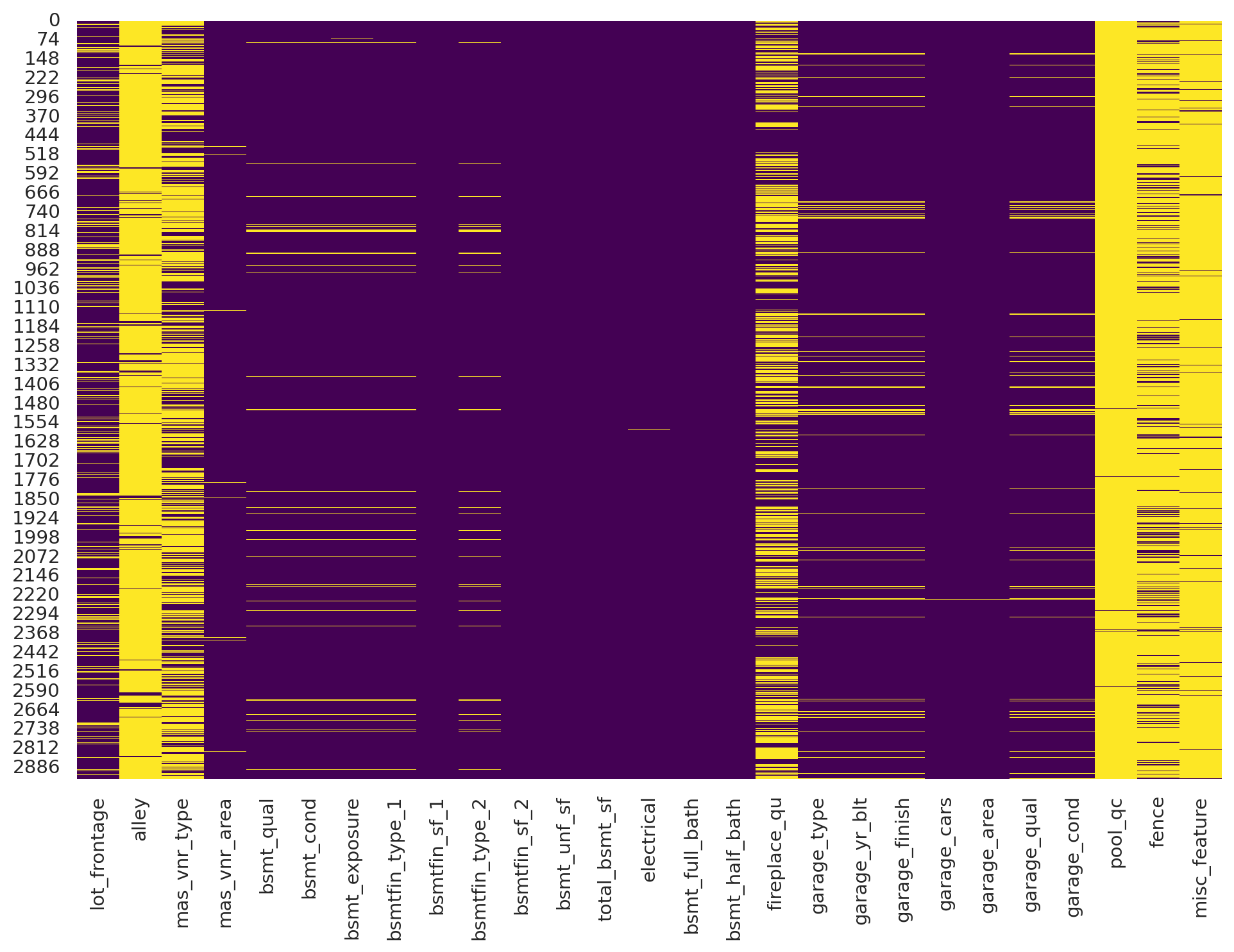
Visualizing Missingness

Sometimes visualizations help identify patterns in missing values. One thing I often do is print a heatmap of my dataframe to get a feel for where my missing values are. We’ll get into data visualization in future lessons but for now here is an example using the searborn library. We can see that several variables have a lot of missing values (alley, fireplace_qu, pool_qc, fence, misc_feature).

import seaborn as sns
sns.set(rc={'figure.figsize':(12, 8)})

ames_missing = ames[missing[missing].index]
sns.heatmap(ames_missing.isnull(), cmap='viridis', cbar=False);

Filling Missing Values (Imputation)

Since we can’t drop all missing values in this data set (since it leaves us with no rows), we need to impute (“fill”) them in. There are several approaches we can use to do this; one of which uses the .fillna() method. This method has various options for filling, you can use a fixed value, the mean of the column, the previous non-nan value, etc:

import numpy as np

# example DataFrame with missing values
df = pd.DataFrame([[np.nan, 2, np.nan, 0],
                   [3, 4, np.nan, 1],
                   [np.nan, np.nan, np.nan, 5],
                   [np.nan, 3, np.nan, 4]],
                  columns=list('ABCD'))
df

	A	B	C	D
0	NaN	2.0	NaN	0
1	3.0	4.0	NaN	1
2	NaN	NaN	NaN	5
3	NaN	3.0	NaN	4

df.fillna(0)  # fill with 0

	A	B	D
0	0.0	2.0	0
1	3.0	4.0	1
2	0.0	0.0	5
3	0.0	3.0	4

df.fillna(df.mean())  # fill with the mean

	A	B	C	D
0	3.0	2.0	NaN	0
1	3.0	4.0	NaN	1
2	3.0	3.0	NaN	5
3	3.0	3.0	NaN	4

df.bfill()  # backward (upwards) fill from non-nan values

	A	B	C	D
0	3.0	2.0	NaN	0
1	3.0	4.0	NaN	1
2	NaN	3.0	NaN	5
3	NaN	3.0	NaN	4

df.ffill()  # forward (downward) fill from non-nan values

	A	B	C	D
0	NaN	2.0	NaN	0
1	3.0	4.0	NaN	1
2	3.0	4.0	NaN	5
3	3.0	3.0	NaN	4

Applying custom functions

There will be times when you want to apply a function that is not built-in to Pandas. For this, we have methods:

df.apply(), applies a function column-wise or row-wise across a dataframe (the function must be able to accept/return an array)
df.applymap(), applies a function element-wise (for functions that accept/return single values at a time)
series.apply()/series.map(), same as above but for Pandas series

For example, say you had the following custom function that defines if a home is considered a luxery home simply based on the price sold.

Don’t worry, you’ll learn more about writing your own functions in future lessons!

def is_luxery_home(x):
    if x > 500000:
        return 'Luxery'
    else:
        return 'Non-luxery'

ames['saleprice'].apply(is_luxery_home)

0       Non-luxery
1       Non-luxery
2       Non-luxery
3       Non-luxery
4       Non-luxery
           ...    
2925    Non-luxery
2926    Non-luxery
2927    Non-luxery
2928    Non-luxery
2929    Non-luxery
Name: saleprice, Length: 2930, dtype: object

This may have been better as a lambda function, which is just a shorter approach to writing functions. This may be a bit confusing but we’ll talk more about lambda functions in the writing functions lesson. For now, just think of it as being able to write a function for single use application on the fly.

ames['saleprice'].apply(lambda x: 'Luxery' if x > 500000 else 'Non-luxery')

0       Non-luxery
1       Non-luxery
2       Non-luxery
3       Non-luxery
4       Non-luxery
           ...    
2925    Non-luxery
2926    Non-luxery
2927    Non-luxery
2928    Non-luxery
2929    Non-luxery
Name: saleprice, Length: 2930, dtype: object

You can even use functions that require additional arguments. Just specify the arguments in .apply():

def is_luxery_home(x, price):
    if x > price:
        return 'Luxery'
    else:
        return 'Non-luxery'

ames['saleprice'].apply(is_luxery_home, price=200000)

0           Luxery
1       Non-luxery
2       Non-luxery
3           Luxery
4       Non-luxery
           ...    
2925    Non-luxery
2926    Non-luxery
2927    Non-luxery
2928    Non-luxery
2929    Non-luxery
Name: saleprice, Length: 2930, dtype: object

Sometimes we may have a function that we want to apply to every element across multiple columns. For example, say we wanted to convert several of the square footage variables to be represented as square meters. For this we can use the .applymap() method.

def convert_to_sq_meters(x):
    return x*0.092903

ames[['gr_liv_area', 'garage_area', 'lot_area']].map(convert_to_sq_meters)

	gr_liv_area	garage_area	lot_area
0	153.847368	49.052784	2946.883160
1	83.241088	67.819190	1075.073516
2	123.468087	28.985736	1320.801951
3	196.025330	48.495366	1032.152330
4	151.338987	44.779246	1280.203340
...	...	...	...
2925	93.181709	54.626964	732.725961
2926	83.798506	44.965052	820.798005
2927	90.115910	0.000000	965.355073
2928	129.042267	38.833454	925.313880
2929	185.806000	60.386950	889.732031

2930 rows × 3 columns

10.8 Chapter Summary

In this chapter, you learned how to manipulate columns in a pandas DataFrame — a foundational skill for any kind of data analysis or modeling. You practiced working with both numeric and non-numeric data and explored common data wrangling tasks that analysts use every day.

Here’s a recap of what you learned:

How to rename columns using .rename() or string methods like .str.lower() and .str.replace()
How to create new columns by performing arithmetic with scalars or other columns
How to remove columns using .drop()
How to work with text data, including string concatenation and using the .str accessor
How to replace values using a mapping (via .replace())
How to detect and handle missing values using .isnull(), .dropna(), and .fillna()
How to apply custom functions to transform your data using .apply() and .applymap()

These skills form the building blocks of effective data cleaning and transformation.

In the next few chapters, we’ll build on this foundation and introduce even more essential data wrangling techniques, including:

Computing summary statistics and descriptive analytics
Grouping and aggregating data
Joining multiple datasets
Reshaping data with pivot tables and the .melt() and .pivot() methods

By the end of these upcoming lessons, you’ll be well-equipped to clean, prepare, and explore real-world datasets using pandas.

10.9 Exercise: Heart Disease Data

In this exercise, you’ll apply what you’ve learned in this chapter to a new dataset on heart disease, which includes various patient health indicators that may be predictive of cardiovascular conditions.

Read more about this dataset on Kaggle, and you can download copy of the heart.csv file here.

Your task is to perform several data wrangling steps to start cleaning and transforming this dataset.

Import the Data

Load the dataset into a DataFrame using pd.read_csv().
Preview the first few rows with .head().

Clean the Column Names

Check out the column names and think how you would standardize these names. Use .columns and string methods to:

Convert all column names to lowercase
Replace any spaces or dashes with underscores
Remove any trailing or leading whitespace

Handle Missing Values

Check for missing values using .isnull().sum().
If any columns contain missing values:
- Identify the mode (most frequent value) for those columns
- Fill the missing values using .fillna()

The mode can be accessed with .mode().iloc[0] to retrieve the most frequent value.

Create a New Column

Create a new column called risk, calculated as:

\[ \text{risk} = \frac{\text{age}}{\text{rest\_bp} + \text{chol} + \text{max\_hr}} \]

Be sure to use parentheses in your formula to ensure proper order of operations.

Replace Values in a Categorical Column

The rest_ecg column contains several text categories. Recode the values using .replace() and the following mapping:

Original Value	New Value
normal	normal
left ventricular hypertrophy	lvh
ST-T wave abnormality	stt_wav_abn

Make sure to overwrite the existing column with the updated values.

The Ames Housing Data

10.1 Renaming Columns

Renaming Specific Columns

Renaming Many Columns at Once

Knowledge Check

10.2 Performing Calculations with Columns

10.3 Adding and Removing Columns

Adding Columns

Removing Columns

Knowledge check

10.4 Overwriting columns

10.5 Calculating with Multiple Columns

Combining Multiple Operations

Knowledge check

10.6 Working with String Columns

String Concatenation

String Methods with .str

10.7 More Complex Column Manipulation

Replacing Values

Missing values

Dropping Missing Values

Visualizing Missingness

Filling Missing Values (Imputation)

Applying custom functions

10.8 Chapter Summary

10.9 Exercise: Heart Disease Data

String Methods with `.str`