28 Cross-validation: Reliable model evaluation

Let’s start with an uncomfortable truth: we’ve been breaking a fundamental rule of machine learning throughout Chapters 25-27. Remember back in Module 8 when you learned the golden rule: “Don’t touch the test set until you’ve selected your final model”? Well, every time you compared different max_depth values, tuned hyperparameters, or selected between models based on test set performance, you were peeking at the test set—and each peek made your test scores less trustworthy.

This isn’t a criticism of what you’ve learned so far. In fact, understanding the simple train/test split was an essential foundation. But now you’re ready for the professional approach that data scientists use in production: cross-validation. This technique solves a critical problem: how do you honestly compare models and tune hyperparameters without contaminating your test set?

Experiential learning

Imagine you’re studying for an exam. Your professor gives you a practice test to help you prepare. You take it, see which questions you got wrong, study those topics more, and take the practice test again. You repeat this several times, adjusting your studying based on the practice test results.

Now imagine your professor uses that same practice test as the actual exam. Your score would be artificially inflated—it wouldn’t reflect how well you’d perform on truly new questions. You’ve essentially “overfit” to that specific practice test.

This is exactly what happens when you repeatedly use test set performance to guide modeling decisions. By the end of this chapter, you’ll learn how cross-validation gives you unlimited “practice tests” while keeping your final exam (test set) pristine and trustworthy.

This chapter addresses a crucial gap between textbook theory and real-world practice. You’ll learn why the simple workflows from previous chapters were pedagogically useful but need refinement for production work, and more importantly, you’ll learn the proper workflow that ensures your model performance estimates are honest and reliable.

By the end of this chapter, you will be able to:

Explain why repeatedly evaluating models on the test set leads to test set contamination and optimistically biased performance estimates
Describe how cross-validation solves the validation problem by rotating through different subsets of the training data
Visualize and explain how k-fold cross-validation works, including how data is split and how models are trained/validated across folds
Implement cross-validation in scikit-learn using cross_val_score() for single metrics and cross_validate() for multiple metrics
Compare multiple models using cross-validation scores instead of test set performance
Choose appropriate values for k (number of folds) based on dataset size and computational constraints
Interpret cross-validation results, including mean scores and standard deviations across folds
Understand when and why to use stratified cross-validation for classification problems
Apply the five-stage proper workflow: (1) train/test split, (2) CV for model comparison, (3) select best model, (4) retrain on full training set, (5) test set evaluation ONCE
Articulate why this workflow produces trustworthy performance estimates that stakeholders can rely on

Follow along in Colab

As you read through this chapter, we encourage you to follow along using the companion notebook in Google Colab (or another editor of your choice). This interactive notebook lets you run all the code examples covered here—and experiment with your own ideas.

👉 Open the Cross-Validation Notebook in Colab.

28.1 The test set dilemma: What we’ve been doing

Let’s trace back through what you’ve learned and practiced over the past few chapters. In Module 8, you learned the fundamental train/test split workflow:

# Example workflow pattern (X, y, and model would need to be defined)
from sklearn.model_selection import train_test_split

# Split data into train and test sets
X_train, X_test, y_train, y_test = train_test_split(
    X, y, test_size=0.3, random_state=42
)

# Train on training set
model.fit(X_train, y_train)

# Evaluate on test set ONCE at the end
test_score = model.score(X_test, y_test)

The logic was clear and sensible:

Training set: Where your model learns patterns
Test set: Completely held-out data to evaluate how well patterns generalize
Critical rule: Don’t touch the test set until you’ve made all your modeling decisions

This test set acts as a proxy for future, unseen data. If your model performs well on the test set, you can be confident it will perform well in production.

The peeking problem

But then in Chapters 21-27, you started building real models and facing real decisions. And here’s where theory met practice:

Chapter 25 (Decision Trees): You needed to choose a good value for max_depth. So naturally, you tried several options:

######################################
# Psuedocode: For demonstration only #
######################################

# Try shallow tree
dt_shallow = DecisionTreeClassifier(max_depth=3)
dt_shallow.fit(X_train, y_train)
score_shallow = dt_shallow.score(X_test, y_test)  # ← First peek!

# Try deeper tree
dt_deep = DecisionTreeClassifier(max_depth=10)
dt_deep.fit(X_train, y_train)
score_deep = dt_deep.score(X_test, y_test)  # ← Second peek!

# Compare and choose the winner
if score_deep > score_shallow:
    best_model = dt_deep  # Chose based on test set performance

Chapter 26 (Random Forests): You wanted to tune hyperparameters, so you evaluated different configurations:

######################################
# Psuedocode: For demonstration only #
######################################

# Try default Random Forest
rf_default = RandomForestClassifier()
rf_default.fit(X_train, y_train)
score_default = rf_default.score(X_test, y_test)  # ← Another peek

# Try tuned version
rf_tuned = RandomForestClassifier(n_estimators=300, max_depth=20)
rf_tuned.fit(X_train, y_train)
score_tuned = rf_tuned.score(X_test, y_test)  # ← Yet another peek

# Keep the better one
best_model = rf_tuned if score_tuned > score_default else rf_default

Each evaluation felt necessary—how else would you make informed decisions?

The core problem

But here’s the problem: every time you used test set performance to make a decision, you implicitly incorporated information from the test set into your model selection process.

Why peeking matters

Think about what’s really happening when you repeatedly evaluate on the test set:

Try model A → test accuracy = 85%
Try model B → test accuracy = 87%
Try model C → test accuracy = 86%
Choose model B because it scored highest on the test set
Report “test accuracy” = 87%

But is that 87% an honest estimate of performance on truly new data? No! You selected model B specifically because it happened to perform best on this particular test set. Model B might have just gotten lucky with these specific test observations.

Test set contamination

Once you’ve used test set performance to make decisions, that test set is “contaminated”—it’s no longer a pure measure of generalization. You’ve essentially tuned your model selection to this specific test set, which is a subtle form of overfitting.

The consequence: Your reported test performance is optimistically biased. It will likely be higher than the true performance you’ll see on genuinely new data in production.

This is similar to the studying-for-an-exam analogy: if you see the exam questions beforehand and adjust your studying accordingly, your exam score won’t accurately reflect your knowledge—it’ll be inflated by your exposure to those specific questions.

A realistic scenario

Let’s make this concrete with a realistic example that demonstrates exactly how test set contamination happens in practice.

Imagine you’re building a customer churn prediction model for a subscription-based business. You have 1,000 customers in your dataset, and you want to find the best random forest configuration by trying different combinations of n_estimators and max_depth. This is a completely normal modeling task—you need to explore the hyperparameter space to find what works best.

The problem is, if you evaluate each of these 20 configurations on your test set to decide which is “best,” you’re peeking at the test set 20 times. By the end of this process, you’ve selected a configuration specifically because it performed well on these particular test observations. Some of that performance is genuine model quality, but some is just random luck—the model happened to align well with the quirks of this specific test set.

Let’s see this in action:

Data preparation: Create customer churn dataset

from sklearn.datasets import make_classification
from sklearn.model_selection import train_test_split
from sklearn.ensemble import RandomForestClassifier

# Create synthetic customer churn dataset
X, y = make_classification(
    n_samples=1000,
    n_features=10,
    n_informative=8,
    n_redundant=2,
    n_classes=2,
    weights=[0.8, 0.2],  # 20% churn rate
    random_state=42
)

# Train/test split
X_train, X_test, y_train, y_test = train_test_split(
    X, y, test_size=0.3, random_state=42, stratify=y
)

# You're building a customer churn prediction model
# You try 20 different hyperparameter combinations
best_test_score = 0
best_config = None

for n_estimators in [50, 100, 200, 300]:
    for max_depth in [5, 10, 15, 20, None]:
        rf = RandomForestClassifier(
            n_estimators=n_estimators,
            max_depth=max_depth,
            random_state=42
        )
        rf.fit(X_train, y_train)
        test_score = rf.score(X_test, y_test)  # Peeking 20 times!

        if test_score > best_test_score:
            best_test_score = test_score
            best_config = (n_estimators, max_depth)

print(f"Best config: {best_config}")
print(f"Test accuracy: {best_test_score:.3f}")  # Is this trustworthy?

Best config: (300, 20)
Test accuracy: 0.910

The result: When you deploy this model in production, you might see something like:

Test set accuracy (during development): 91%
Production accuracy (on new customers): 85%

That 6-percentage-point drop is partly because you overfit to the test set through repeated evaluation. Your test score gave you false confidence.

But we had to make decisions somehow

This might feel frustrating. You had legitimate questions that needed answers:

Which max_depth value works best?
Should I use 100 or 300 trees in my Random Forest?
Does adding this feature improve performance?
Which model architecture performs best?

You couldn’t answer these questions without evaluating somewhere. So what’s the solution?

Cross-validation to the rescue!

This is precisely the dilemma that cross-validation solves. It gives you a way to answer all these questions—to compare, tune, and select—without ever touching your test set. Let’s see how.

28.2 The ideal solution: A three-way split

Before we get to cross-validation, let’s understand the ideal (but not always practical) solution: splitting your data into three parts instead of two.

Train, validation, and test sets

The proper workflow should look like this:

Full Dataset
    ↓
    ├─── Training Set (60%)      ← Build models here
    ├─── Validation Set (20%)    ← Compare models here
    └─── Test Set (20%)          ← Final evaluation ONCE

Each portion has a distinct purpose:

Training set: This is where your models learn. You fit models using only this data.
Validation set: This is your “practice exam”—you can look at it as many times as you want during development. Use it to:
- Compare different models
- Tune hyperparameters
- Select features
- Make any other modeling decisions
Test set: This remains completely locked away until the very end. You evaluate your final chosen model on it exactly once to get an honest estimate of production performance.

The workflow in practice

Here’s how the three-way split workflow operates:

flowchart TD
    A["📊 Complete Dataset<br/>(1000 observations)"] --> B["Split into 3 parts"]

    B --> C["🎯 Training Set<br/>60% (600 obs)<br/><br/>Purpose: Build models"]
    B --> D["🔍 Validation Set<br/>20% (200 obs)<br/><br/>Purpose: Compare & tune"]
    B --> E["🔒 Test Set<br/>20% (200 obs)<br/><br/>Purpose: Final evaluation"]

    C --> F["Model Development Phase"]

    F --> G["Try Model 1<br/>Train on Training Set"]
    F --> H["Try Model 2<br/>Train on Training Set"]
    F --> I["Try Model 3<br/>Train on Training Set"]
    F --> J["Try Model 4<br/>Train on Training Set"]

    G --> K["Evaluate on<br/>Validation Set"]
    D --> K
    H --> K
    I --> K
    J --> K

    K --> L["Select Best Model<br/>based on validation scores"]

    L --> M["Retrain best model<br/>on full Training Set"]

    E --> N["Final Evaluation Phase"]
    M --> N

    N --> O["🎉 Evaluate ONCE on Test Set<br/>Get trustworthy performance estimate"]

    style A fill:#e1f5fe
    style C fill:#c8e6c9
    style D fill:#fff9c4
    style E fill:#ffccbc
    style F fill:#f3e5f5
    style K fill:#fff9c4
    style L fill:#c8e6c9
    style O fill:#c8e6c9

Key points illustrated above:

Training set (60%): Used repeatedly to train different model candidates
Validation set (20%): Used repeatedly to compare and select among models—this prevents test set contamination
Test set (20%): Locked away and used exactly once at the end for final, honest evaluation

This solves the contamination problem perfectly. You can peek at the validation set as many times as you want—try hundreds of models if you like—without compromising the integrity of your test set.

The catch: Data efficiency

This approach is conceptually perfect but has a practical problem: it requires splitting your data into three parts, which can leave you with insufficient data for each purpose.

Consider a medium-sized dataset with 1,000 observations:

1,000 total observations
    ├─── Training: 600 observations
    ├─── Validation: 200 observations
    └─── Test: 200 observations

Now you’re only training on 600 observations when you could have used 800 (if you didn’t need a separate validation set). For many real-world problems, especially with limited data, this sacrifice is significant:

Fewer training examples can hurt model performance—you’re not giving your model enough data to learn patterns effectively
Smaller validation set might give unreliable estimates—200 observations might not be representative, leading to poor model selection
Smaller test set also reduces reliability of your final evaluation

When data is scarce

With small-to-medium datasets (thousands of observations, not millions), the three-way split can be wasteful. You want to use as much data as possible for training while still maintaining honest evaluation.

This tension—needing validation without sacrificing training data—is what makes cross-validation so valuable.

The question becomes: Is there a way to get the benefits of a validation set without actually reserving a separate portion of data? The answer is yes, and it’s called cross-validation.

28.3 Cross-validation: The clever solution

Cross-validation is one of the most elegant ideas in machine learning. It solves both problems at once: it gives you honest performance estimates (like a validation set) while using your data efficiently (not wasting observations on a separate validation set).

The big idea

Here’s the key insight: what if, instead of holding out one fixed validation set, we rotate which portion of the training data acts as validation? With cross-validation, you never create a separate validation set. Instead, you:

Keep your test set completely separate (just like before)
Within your training set, temporarily designate different portions as “validation” in rotation
Each observation gets used for both training and validation (just at different times)

The workflow looks like this:

Full Dataset
    ↓
    ├─── Training Set (80%)    ← Use for BOTH training AND validation via CV
    └─── Test Set (20%)        ← Keep locked away until the end

Notice you only split once (train/test), not twice (train/val/test). The magic happens within the training set through a process called k-fold cross-validation.

How k-fold cross-validation works

The term “k-fold” refers to dividing your training data into k equal-sized pieces (called “folds”). The letter k is simply a number you choose—typically 5 or 10—that determines how many pieces to split your training data into.

Here’s the brilliant part: instead of setting aside one fixed portion of your training data as a validation set (which you’d never use for training), k-fold cross-validation rotates which fold acts as the validation set. Each fold gets a turn being the validation set while the remaining folds are used for training. This means:

Every observation in your training set gets used for validation exactly once
Every observation gets used for training in k-1 iterations
You end up with k different performance estimates that you can average together

This rotation strategy maximizes data efficiency (you’re using more data for training than with a fixed validation set) while still providing honest performance estimates (each validation fold is held out during its evaluation).

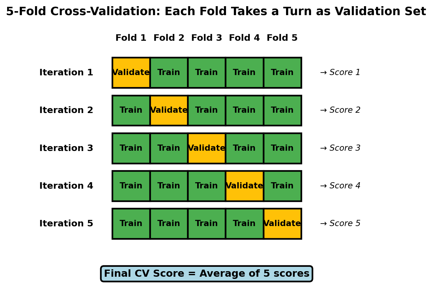
Let’s walk through a concrete example using 5-fold CV (k=5), which is the most common choice:

Visual representation of 5-fold cross-validation showing how each fold takes a turn as the validation set

What’s happening in this visualization:

Initial split: The training set is divided into 5 equal-sized folds (shown across the top)
Rotation pattern: In each of the 5 iterations (rows):
- One fold serves as the validation set (amber/yellow)
- The remaining four folds serve as the training set (green)
- Each iteration produces one validation score
Data efficiency: Notice that every fold is used for training in 4 out of 5 iterations (80% utilization) and for validation in 1 out of 5 iterations
Final estimate: The 5 validation scores are averaged to produce the final cross-validation score—a reliable estimate of model performance

Why this is brilliant

Cross-validation achieves several goals simultaneously:

The magic of CV

Data efficiency: Every observation in your training set gets used for training (in 4 out of 5 folds). You’re training on 80% of your training set each time, not just 60%.

Robust validation: Every observation also gets used for validation (in 1 out of 5 folds). You’re validating on different portions of data, so your performance estimate is based on the entire training set.

Multiple evaluations: You get 5 different performance estimates from 5 different validation splits, then average them. This is much more reliable than a single validation score from a fixed validation set.

Variance estimates: The variation across folds tells you how stable your model is. High variation suggests your model’s performance is sensitive to which data it’s trained on.

Test set remains pristine: All of this happens within the training set. Your test set is never touched, so it remains a completely honest final evaluation.

Let’s make this concrete with an example:

from sklearn.model_selection import cross_val_score
from sklearn.ensemble import RandomForestClassifier

# Assume X_train, y_train from your train/test split
# Test set (X_test, y_test) remains untouched

# Create a model
rf = RandomForestClassifier(n_estimators=100, random_state=42)

# Perform 5-fold cross-validation on training set
cv_scores = cross_val_score(rf, X_train, y_train, cv=5, scoring='accuracy')

print(f"Fold scores: {cv_scores}")
print(f"Mean CV accuracy: {cv_scores.mean():.3f}")
print(f"Std deviation: {cv_scores.std():.3f}")

Output might look like:

Fold scores: [0.867 0.883 0.875 0.892 0.858]
Mean CV accuracy: 0.875
Std deviation: 0.012

You’ve now evaluated your model on the training set 5 different ways, getting a robust performance estimate (87.5% ± 1.2%) without ever touching the test set.

Comparing to the validation set approach

Let’s contrast the two approaches side-by-side to see why cross-validation is more efficient:

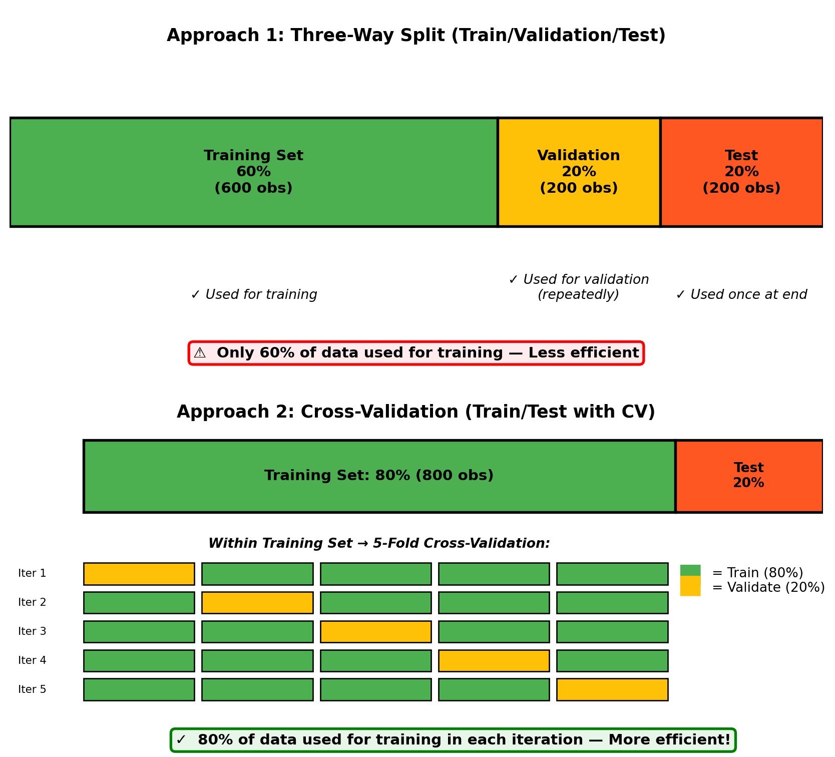
Comparison of three-way split vs. cross-validation approaches, showing data efficiency

Key differences highlighted:

Data efficiency:
- Three-way split uses only 60% of data for training (400 fewer observations)
- Cross-validation uses 80% of data for training in each fold (maximizes learning)
Validation robustness:
- Three-way split relies on a single fixed validation set (200 observations)
- Cross-validation averages across 5 different validation sets (all 800 training observations participate)
Flexibility:
- Three-way split: Once you set aside 200 observations for validation, you can never use them for training
- Cross-validation: Every observation contributes to both training and validation (just at different times)

The cross-validation approach gives you the best of both worlds: honest performance estimates AND efficient use of your limited data.

28.4 Proper workflow: What we should have done

Now that you understand cross-validation, here’s the proper pattern you’ll use going forward when comparing models or tuning hyperparameters:

The proper workflow template

Create train/test split and lock the test set away
Compare models using cross-validation on training set ONLY
Select best model based on CV scores (not test scores!)
Retrain best model on all training data
Evaluate on test set EXACTLY ONCE

######################################
# Psuedocode: For demonstration only #
######################################
from sklearn.model_selection import train_test_split, cross_val_score

# Step 1: Split and lock test set
X_train, X_test, y_train, y_test = train_test_split(
    X, y, test_size=0.2, random_state=42, stratify=y
)

# Step 2: Compare models using CV on training set
model1 = SomeModel(params1)
model2 = SomeModel(params2)

cv_scores1 = cross_val_score(model1, X_train, y_train, cv=5)
cv_scores2 = cross_val_score(model2, X_train, y_train, cv=5)

# Step 3: Select best based on CV
best_model = model1 if cv_scores1.mean() > cv_scores2.mean() else model2

# Step 4: Retrain on all training data
best_model.fit(X_train, y_train)

# Step 5: Evaluate on test set ONCE
final_test_score = best_model.score(X_test, y_test)

Key point: All model comparisons and hyperparameter tuning use CV on the training set. The test set is only touched once at the very end, making the final test score a trustworthy estimate of production performance.

28.5 Implementing cross-validation in scikit-learn

Now that you understand the conceptual foundation, let’s dive into the practical details of implementing cross-validation using scikit-learn. The library provides several functions and options to fit different needs.

For the examples in this section, we’ll use the Default dataset from ISLP, that we’ve seen in previous chapters:

Code

import pandas as pd
from ISLP import load_data
from sklearn.model_selection import train_test_split

# Load the Default dataset
Default = load_data('Default')

# Prepare features and target
X = pd.get_dummies(Default[['balance', 'income', 'student']], drop_first=True)
y = (Default['default'] == 'Yes').astype(int)

# Create train/test split (lock away test set)
X_train, X_test, y_train, y_test = train_test_split(
    X, y, test_size=0.2, random_state=42, stratify=y
)

print(f"Training set: {len(X_train)} observations")
print(f"Test set: {len(X_test)} observations")
print(f"Default rate: {y_train.mean():.1%}")

Training set: 8000 observations
Test set: 2000 observations
Default rate: 3.3%

Basic usage: `cross_val_score()`

The simplest and most common function is cross_val_score(), which performs k-fold CV and returns the scores from each fold:

from sklearn.model_selection import cross_val_score
from sklearn.ensemble import RandomForestClassifier

# Create your model
model = RandomForestClassifier(n_estimators=100, random_state=42)

# Perform 5-fold cross-validation
cv_scores = cross_val_score(
    estimator=model,        # Your model
    X=X_train,             # Training features
    y=y_train,             # Training labels
    cv=5,                  # Number of folds
    scoring='accuracy'     # Metric to compute
)

print(f"Fold scores: {cv_scores}")
print(f"Mean: {cv_scores.mean():.3f}")
print(f"Std Dev: {cv_scores.std():.3f}")

Fold scores: [0.966875 0.970625 0.9675   0.973125 0.970625]
Mean: 0.970
Std Dev: 0.002

Each value represents the accuracy on one validation fold. The mean gives you the overall estimate, and the standard deviation tells you how variable the performance is across folds.

Choosing scoring metrics

The scoring parameter determines what metric to compute. The appropriate choice depends on your problem type.

You can find all the available scoring metrics here: https://scikit-learn.org/stable/modules/model_evaluation.html#string-name-scorers

For classification:

# Accuracy (default for classifiers)
cross_val_score(model, X_train, y_train, cv=5, scoring='accuracy')

# F1 score (good for imbalanced classes)
cross_val_score(model, X_train, y_train, cv=5, scoring='f1')

# ROC AUC (measures ranking quality)
cross_val_score(model, X_train, y_train, cv=5, scoring='roc_auc')

# Precision and recall
cross_val_score(model, X_train, y_train, cv=5, scoring='precision')
cross_val_score(model, X_train, y_train, cv=5, scoring='recall')

For regression:

# R² score (default for regressors)
cross_val_score(model, X_train, y_train, cv=5, scoring='r2')

# Negative mean squared error
cross_val_score(model, X_train, y_train, cv=5, scoring='neg_mean_squared_error')

# Negative mean absolute error
cross_val_score(model, X_train, y_train, cv=5, scoring='neg_mean_absolute_error')

Why “negative” for error metrics?

Scikit-learn’s CV functions are designed to maximize scores. Since lower errors are better, scikit-learn returns negative errors so that “higher is better” remains consistent. Just remember:

neg_mean_squared_error = -5.2 means MSE is actually 5.2
More negative is worse (larger error)
Less negative is better (smaller error)

Advanced: `cross_validate()` for multiple metrics

If you want to compute multiple metrics at once, or get more detailed information, use cross_validate():

from sklearn.model_selection import cross_validate

# Evaluate multiple metrics simultaneously
cv_results = cross_validate(
    model, X_train, y_train,
    cv=5,
    scoring=['accuracy', 'f1', 'roc_auc'],  # Multiple metrics
    return_train_score=True                  # Also get training scores
)

# Results is a dictionary with arrays for each metric
print(f"CV accuracy: {cv_results['test_accuracy'].mean():.3f}")
print(f"CV F1: {cv_results['test_f1'].mean():.3f}")
print(f"CV ROC AUC: {cv_results['test_roc_auc'].mean():.3f}")
print(f"\nTraining accuracy: {cv_results['train_accuracy'].mean():.3f}")

CV accuracy: 0.970
CV F1: 0.418
CV ROC AUC: 0.887

Training accuracy: 1.000

This is useful for:

Comparing multiple metrics at once
Detecting overfitting (comparing train vs. test scores)
Analyzing fit time and score time across folds

Practical example: Comparing models with CV

Now let’s put everything together in a realistic scenario: you have multiple candidate models and need to determine which one performs best. This is one of the most common use cases for cross-validation in practice.

In this example, we’ll compare three different classification algorithms—Logistic Regression, Decision Tree, and Random Forest—to see which handles our data best. Rather than evaluating each on the test set (which would contaminate it), we’ll use 5-fold cross-validation on the training set to get honest performance estimates.

Data preparation: Create customer churn dataset

import numpy as np
from sklearn.datasets import make_classification
from sklearn.model_selection import train_test_split

# Create synthetic data with non-linear patterns
X, y = make_classification(
    n_samples=1000,
    n_features=10,
    n_informative=8,
    n_redundant=0,
    n_clusters_per_class=3,  # Creates non-linear decision boundaries
    flip_y=0.1,  # Adds some noise
    class_sep=0.5,  # Moderate class separation
    random_state=42
)

# Add polynomial interactions to create non-linear relationships
# This will favor tree-based models over linear models
X_poly = np.column_stack([
    X,
    X[:, 0] * X[:, 1],  # Interaction term
    X[:, 2] ** 2,        # Squared term
    X[:, 3] * X[:, 4]    # Another interaction
])

# Train/test split (lock away test set)
X_train, X_test, y_train, y_test = train_test_split(
    X_poly, y, test_size=0.2, random_state=42, stratify=y
)

print(f"Training set: {len(X_train)} observations")
print(f"Test set: {len(X_test)} observations (locked away)")
print(f"Features: {X_train.shape[1]}")

Training set: 800 observations
Test set: 200 observations (locked away)
Features: 13

Now we’ll compare our candidate models using cross-validation. Notice how we never touch the test set during this comparison phase:

from sklearn.model_selection import cross_val_score
from sklearn.tree import DecisionTreeClassifier
from sklearn.ensemble import RandomForestClassifier
from sklearn.linear_model import LogisticRegression

# Define models to compare
models = {
    'Logistic Regression': LogisticRegression(max_iter=1000, random_state=42),
    'Decision Tree': DecisionTreeClassifier(max_depth=10, random_state=42),
    'Random Forest': RandomForestClassifier(n_estimators=100, random_state=42)
}

# Evaluate each with 5-fold CV
print("Model Comparison (5-fold CV on training set):")
print("="*70)

for name, model in models.items():
    # Compute CV scores
    cv_scores = cross_val_score(
        model, X_train, y_train,
        cv=5,
        scoring='roc_auc'  # Using ROC AUC for this example
    )

    mean_score = cv_scores.mean()
    std_score = cv_scores.std()

    print(f"{name:25s} {mean_score:.4f} (±{std_score:.4f})")

print("="*70)

Model Comparison (5-fold CV on training set):
======================================================================
Logistic Regression       0.6451 (±0.0453)
Decision Tree             0.6277 (±0.0758)
Random Forest             0.7760 (±0.0494)
======================================================================

We can see that the random forest model significantlyl outperforms the logistic regression and decision tree models.

Key observations from this example:

We evaluated 3 models using cross-validation, getting reliable performance estimates
The test set was never touched during model comparison
Random Forest appears to be the best performer (highest mean ROC AUC)
The standard deviations are small, indicating consistent performance across folds
Based on these CV results, we’d select Random Forest as our final model

This pattern—define models, evaluate with CV, compare results—is the foundation of professional model development.

28.6 The complete proper workflow

Now that you understand cross-validation conceptually and practically, let’s formalize the complete workflow you’ll use for nearly every machine learning project. This five-stage process ensures you get honest performance estimates while using your data efficiently.

The five stages are:

Initial Setup: Split data into train/test and lock away the test set
Model Development: Compare models using cross-validation on training set ONLY
Select Best: Choose the best model based on CV scores (not test scores!)
Train Final Model: Retrain the selected model on ALL training data
Final Evaluation: Evaluate on test set EXACTLY ONCE to estimate production performance

The critical insight is that all experimentation happens in stages 2-4 using only the training set. The test set remains untouched until the very end, giving you an unbiased estimate of how your final model will perform on new data.

Let’s see this workflow in action with a complete example using the breast cancer dataset:

from sklearn.datasets import load_breast_cancer
from sklearn.model_selection import train_test_split, cross_val_score
from sklearn.ensemble import RandomForestClassifier
from sklearn.tree import DecisionTreeClassifier
from sklearn.linear_model import LogisticRegression

# Load data
data = load_breast_cancer()
X, y = data.data, data.target

# ========== STEP 1: Initial Setup ==========
print("STEP 1: Initial Setup - Split data and lock away test set")
print("="*60)
X_train, X_test, y_train, y_test = train_test_split(
    X, y, test_size=0.2, random_state=42, stratify=y
)
print(f"Training set: {len(X_train)} samples")
print(f"Test set: {len(X_test)} samples")
print("🔒 Test set locked away\n")

# ========== STEP 2: Model Development ==========
print("STEP 2: Model Development - Compare models using CV")
print("="*60)
models = {
    'Logistic Regression': LogisticRegression(max_iter=10000),
    'Decision Tree': DecisionTreeClassifier(max_depth=10),
    'Random Forest': RandomForestClassifier(n_estimators=100, random_state=42)
}

cv_results = {}
for name, model in models.items():
    cv_scores = cross_val_score(model, X_train, y_train, cv=5)
    cv_results[name] = {
        'mean': cv_scores.mean(),
        'std': cv_scores.std(),
        'model': model
    }
    print(f"{name:25s} {cv_scores.mean():.4f} (±{cv_scores.std():.4f})")

# ========== STEP 3: Select Best ==========
print("\nSTEP 3: Select Best - Choose model with highest CV score")
print("="*60)
best_name = max(cv_results, key=lambda k: cv_results[k]['mean'])
best_model = cv_results[best_name]['model']
print(f"Selected model: {best_name}")

# ========== STEP 4: Train Final Model ==========
print("\nSTEP 4: Train Final Model - Retrain on all training data")
print("="*60)
best_model.fit(X_train, y_train)
print(f"Trained {best_name} on {len(X_train)} training samples")

# ========== STEP 5: Final Evaluation ==========
print("\nSTEP 5: Final Evaluation - Test set evaluation (ONLY ONCE)")
print("="*60)
test_score = best_model.score(X_test, y_test)
print(f"Cross-validation score (training): {cv_results[best_name]['mean']:.4f}")
print(f"Test score (held-out data):        {test_score:.4f}")
print("\n🔓 Test set has now been used - project complete!")

STEP 1: Initial Setup - Split data and lock away test set
============================================================
Training set: 455 samples
Test set: 114 samples
🔒 Test set locked away

STEP 2: Model Development - Compare models using CV
============================================================
Logistic Regression       0.9516 (±0.0112)
Decision Tree             0.9253 (±0.0189)
Random Forest             0.9538 (±0.0235)

STEP 3: Select Best - Choose model with highest CV score
============================================================
Selected model: Random Forest

STEP 4: Train Final Model - Retrain on all training data
============================================================
Trained Random Forest on 455 training samples

STEP 5: Final Evaluation - Test set evaluation (ONLY ONCE)
============================================================
Cross-validation score (training): 0.9538
Test score (held-out data):        0.9561

🔓 Test set has now been used - project complete!

The golden rule

Test set touches: Exactly ONE

If you find yourself evaluating on the test set more than once during model development, stop—you’re contaminating it. Go back to Stage 2 and use cross-validation instead.

This five-stage workflow is now your standard approach for any machine learning project. It ensures honest performance estimates, efficient use of data, and trustworthy models.

28.7 Choosing the right number of folds

The cv parameter controls how many folds to create. The choice involves trade-offs:

Quick guide to selecting k

k=5 (default choice): Use this unless you have a specific reason not to. Trains on 80% per fold, good balance of speed and reliability.
k=10: Use for smaller datasets (< 5K observations) or when you need maximum reliability. Trains on 90% per fold but takes twice as long as k=5.
k=3: Use for very large datasets (> 100K observations) where k=5 is too slow, or for rapid prototyping. Faster but less reliable.

Bottom line: When in doubt, use k=5. The important part is using cross-validation at all rather than repeatedly evaluating on the test set!

These guidelines apply to most situations, but the specific choice may vary based on your computational resources and time constraints. In practice, you’ll rarely go wrong with k=5.

Why we didn’t start with cross-validation

You might wonder: “If CV is the proper approach, why didn’t we learn it in Module 8?”

The answer: Educational scaffolding. Learning complex topics works best when you build foundations first:

Chapter 21: Learn the core concept—separate data for training and testing
Chapters 21-27: Practice building models with simple train/test splits
Chapter 28 (now): Refine to professional standards with cross-validation

By starting simple, you could focus on understanding why we separate data before learning how to do it optimally. Now you have the context to understand why CV matters and the experience to use it effectively. This progression was intentional and puts you ahead of many practitioners who still use the simpler (but problematic) approach.

28.8 Summary

This chapter equipped you with one of the most important skills in professional machine learning: honest model evaluation through cross-validation. The fundamental problem we addressed is test set contamination—repeatedly using the test set to compare models or tune hyperparameters leads to optimistically biased performance estimates. Each time you make a modeling decision based on test set performance, you’re implicitly fitting to the test set, making your test scores unreliable predictors of production performance.

Cross-validation solves this elegantly by creating a validation process entirely within your training set. Instead of setting aside a fixed validation set, k-fold cross-validation rotates through different subsets of the training data, using each fold as a validation set exactly once. This approach provides reliable validation without touching the test set, uses your training data efficiently, and produces robust estimates by averaging performance across multiple folds. In practice, k=5 provides a good balance of speed and reliability for most situations.

The proper workflow you should follow for every machine learning project consists of five stages: (1) split data into train/test and lock away the test set, (2) compare models using cross-validation on the training set only, (3) select the best model based on CV scores, (4) retrain the selected model on all training data, and (5) evaluate on the test set exactly once. This workflow ensures that all experimentation—model comparison, hyperparameter tuning, and feature selection—happens using cross-validation on the training set, keeping your test set pristine until the final evaluation.

In scikit-learn, you’ll use cross_val_score() for single metric evaluation and cross_validate() for multiple metrics simultaneously. For classification problems, scikit-learn automatically applies stratified cross-validation to ensure each fold has representative class distributions, which is especially important for imbalanced datasets.

The Golden Rule of Model Evaluation

Test set touches = EXACTLY ONE

If you evaluate on the test set more than once during model development, you’re contaminating it. All experimentation must happen using cross-validation on the training set. This single principle separates trustworthy machine learning from wishful thinking.

Why does this matter? When you tell stakeholders “this model achieves 95% accuracy,” they need to confidently expect production performance to match your test scores. Proper cross-validation prevents costly surprises, maintains your credibility as a data scientist, and ensures models perform as expected when deployed. This is the foundation of trustworthy, production-ready machine learning.

Now that you know how to properly evaluate models, the next chapter will dive deeper into systematically finding the best hyperparameter configurations through hyperparameter tuning—a process that relies heavily on the cross-validation workflow you just mastered.

28.9 End of chapter exercises

These exercises build on your previous work from Chapters 25-27, asking you to revisit those models using the proper cross-validation workflow you learned in this chapter.

Exercise 1: Fixing the baseball salary predictions

In Chapter 26 Exercise 1, you built random forest models to predict baseball player salaries using the Hitters dataset. You likely compared different models by evaluating them on the test set—which we now know is problematic.

Revisit that analysis properly:

Part A: Identify the problem

Review your original code from Chapter 26 Exercise 1
Count how many times you evaluated models on the test set
Explain why repeatedly using the test set for model comparison is problematic

Part B: Implement proper workflow

Use the same train/test split you used originally (for fair comparison)
Compare at least 4 different model configurations using 5-fold CV on the training set:
- Decision tree with tuned depth
- Random Forest with default parameters
- Random Forest with tuned n_estimators
- Random Forest with tuned max_depth and min_samples_split
For each model, report mean CV score and standard deviation
Select the best model based on CV scores
Train final model on full training set
Evaluate on test set ONCE

Part C: Compare approaches

Compare the “best” test score from your original Chapter 26 work (where you peeked at test set) to the honest test score from the proper workflow
Are they different? If so, explain why
Which estimate would you trust for predicting production performance? Why?

Part D: Check stability

Repeat the CV model comparison using k=3 and k=10
Does the same model win under different k values?
How much do the CV estimates change?
What does this tell you about model stability?

Exercise 2: Proper default risk assessment

In Chapter 26 Exercise 2, you built random forests to predict credit card default using the Default dataset. Now implement the proper evaluation workflow.

Your tasks:

Part A: Clean slate with proper workflow

Start fresh with the Default dataset
Create train/test split (80/20, stratified by default status)
Define 5 different models to compare:
- Logistic Regression (baseline)
- Decision Tree (try two different depths)
- Random Forest (default parameters)
- Random Forest (tuned parameters of your choice)
Use 5-fold stratified CV on training set to evaluate all models
Report results with mean accuracy, precision, recall, and F1 score for each

Part B: Selection and evaluation

Select the best model based on the metric that matters most for credit default prediction (consider: what’s the cost of false positives vs. false negatives?)
Train final model on full training set
Evaluate on test set once
Create a confusion matrix for the test set predictions
Interpret the results: Is the test performance consistent with CV estimates?

Part C: Feature importance revisited

Using your selected model from Part B, calculate feature importance (recall Chapter 27)
Compare the importance rankings when using CV vs. when training on full training set
Are they similar? Why or why not?

Part D: Business communication

Write a one-page memo to the bank’s risk management team explaining:

Which model you selected and why
The expected accuracy in production (and how you know it’s trustworthy)
Which features drive default predictions
Why your estimates are more reliable than if you’d repeatedly used test set

Exercise 3: The Ames housing challenge

Apply the complete proper workflow to the Ames housing dataset (regression).