8 Lesson 3a: Feature engineering
Data preprocessing and engineering techniques generally refer to the addition, deletion, or transformation of data. In this lesson we introduce you to another tidymodels package, recipes, which is designed to help you preprocess your data before training your model. Recipes are built as a series of preprocessing steps, such as:
- converting qualitative predictors to indicator variables (also known as dummy variables),
- transforming data to be on a different scale (e.g., taking the logarithm of a variable),
- transforming whole groups of predictors together, extracting key features from raw variables (e.g., getting the day of the week out of a date variable),
and so on. Although there is an ever-growing number of ways to preprocess your data, we’ll focus on a few common feature engineering steps applied to numeric and categorical data. This will provide you with a foundation of how to perform feature engineering.
8.1 Learning objectives
By the end of this lesson you’ll be able to:
- Explain how to apply feature engineering steps with the recipes package.
- Filter out low informative features.
- Normalize and standardize numeric features.
- Pre-process nominal and ordinal features.
- Combine multiple feature engineering steps into one recipe and train a model with it.
8.2 Prerequisites
For this lesson we’ll use the recipes package with is automatically loaded with tidymodels and we’ll use the ames.csv housing data.
library(tidymodels)
library(tidyverse)

ames_data_path <- here::here("data", "ames.csv")
ames <- readr::read_csv(ames_data_path)
Let’s go ahead and create our train-test split:
8.3 Create a recipe
To get started, let’s create a model recipe that we will build upon and apply in a model downstream. Before training the model, we can use a recipe to create and/or modify predictors and conduct some preprocessing required by the model.
Similar to the fit() function you’ve already seen, the recipe() function has two primary arguments:
- A formula: Any variable on the left-hand side of the tilde (
~) is considered the response variable (here, aSale_Price). On the right-hand side of the tilde are the predictors. Variables may be listed by name, or you can use the dot (.) to indicate all other variables as predictors. - The data: A recipe is associated with the data set used to create the model. This should always be the training set, so
data = ames_trainhere.
Now we can start adding feature engineering steps onto our recipe using the pipe operator and applying specific feature engineering tasks. The sections that follow provide some discussion as to why we apply each feature engineering step and then we demonstrate how to add it to our recipe.
8.4 Numeric features
Pretty much all algorithms will work out of the box with numeric features. However, some algorithms make some assumptions regarding the distribution of our features. If we look at some of our numeric features, we can see that they span across different ranges:
ames_train %>%
   select_if(is.numeric)
## # A tibble: 2,051 × 35
##    Lot_Frontage Lot_Area Year_Built Year_Remod_Add Mas_Vnr_Area
##           <dbl>    <dbl>      <dbl>          <dbl>        <dbl>
##  1           81    11216       2006           2006            0
##  2            0     2998       2000           2000          513
##  3            0    17871       1995           1996            0
##  4           85    10574       2005           2006            0
##  5           50     6000       1939           1950            0
##  6           35     4251       2006           2007            0
##  7           65     8125       1994           1998          258
##  8           80     8480       1947           1950            0
##  9           60     7200       1951           1951            0
## 10            0    12735       1972           1972            0
## # ℹ 2,041 more rows
## # ℹ 30 more variables: BsmtFin_SF_1 <dbl>, BsmtFin_SF_2 <dbl>,
## #   Bsmt_Unf_SF <dbl>, Total_Bsmt_SF <dbl>, First_Flr_SF <dbl>,
## #   Second_Flr_SF <dbl>, Low_Qual_Fin_SF <dbl>, Gr_Liv_Area <dbl>,
## #   Bsmt_Full_Bath <dbl>, Bsmt_Half_Bath <dbl>, Full_Bath <dbl>,
## #   Half_Bath <dbl>, Bedroom_AbvGr <dbl>, Kitchen_AbvGr <dbl>,
## #   TotRms_AbvGrd <dbl>, Fireplaces <dbl>, Garage_Cars <dbl>, …
Moreover, sometimes our numeric features are skewed or contain outliers. For example, our Gr_Liv_Area feature is skewed right where most values are centered around 1200-1500 square feet of living space but there several larger than normal homes (i.e. Gr_Liv_Area > 3000). In fact, if we look at our scatter plot we can see that the right tail of Gr_Liv_Area values is where the largest residuals are.
p1 <- ggplot(ames_train, aes(Gr_Liv_Area)) +
   geom_histogram(bins = 100)

p2 <- ggplot(ames_train, aes(Gr_Liv_Area, Sale_Price)) +
   geom_point() +
   geom_smooth(method = "lm", se = FALSE)

gridExtra::grid.arrange(p1, p2, nrow = 1)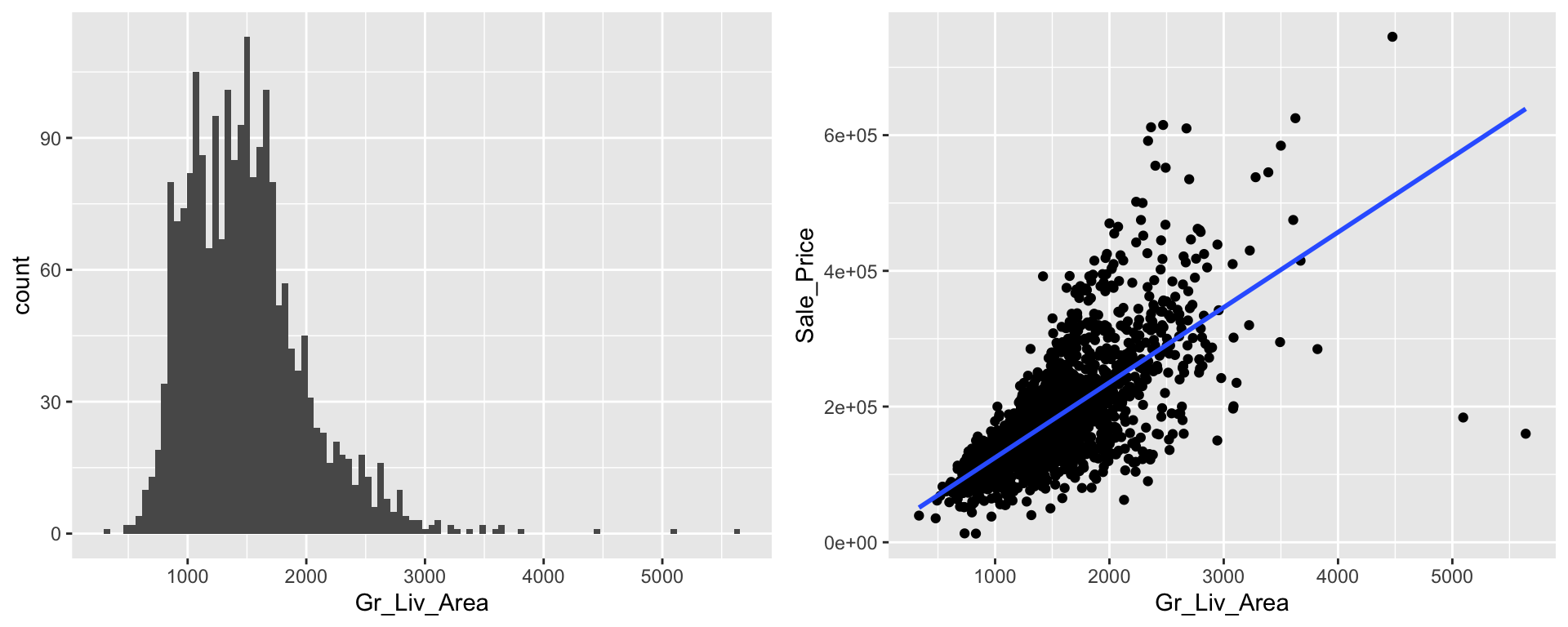
We can incorporate feature engineering steps to help address both of the above concerns.
8.4.1 Standardizing
We should always consider the scale on which the individual features are measured. What are the largest and smallest values across all features and do they span several orders of magnitude? Models that incorporate smooth functions of input features are sensitive to the scale of the inputs. For example, \(5X+2\) is a simple linear function of the input X, and the scale of its output depends directly on the scale of the input. Many algorithms use linear functions within their algorithms, some more obvious (e.g., ordinary least squares and regularized regression) than others (e.g., neural networks, support vector machines, and principal components analysis). Other examples include algorithms that use distance measures such as the Euclidean distance (e.g., k nearest neighbor, k-means clustering, and hierarchical clustering).
For these models and modeling components, it is often a good idea to standardize the features. Standardizing features includes centering and scaling so that numeric variables have zero mean and unit variance, which provides a common comparable unit of measure across all the variables.
Whether or not a machine learning model requires normalization of the features depends on the model family. Linear models such as logistic regression generally benefit from scaling the features while other models such as tree-based models (i.e. decision trees, random forests) do not need such preprocessing (but will not suffer from it).
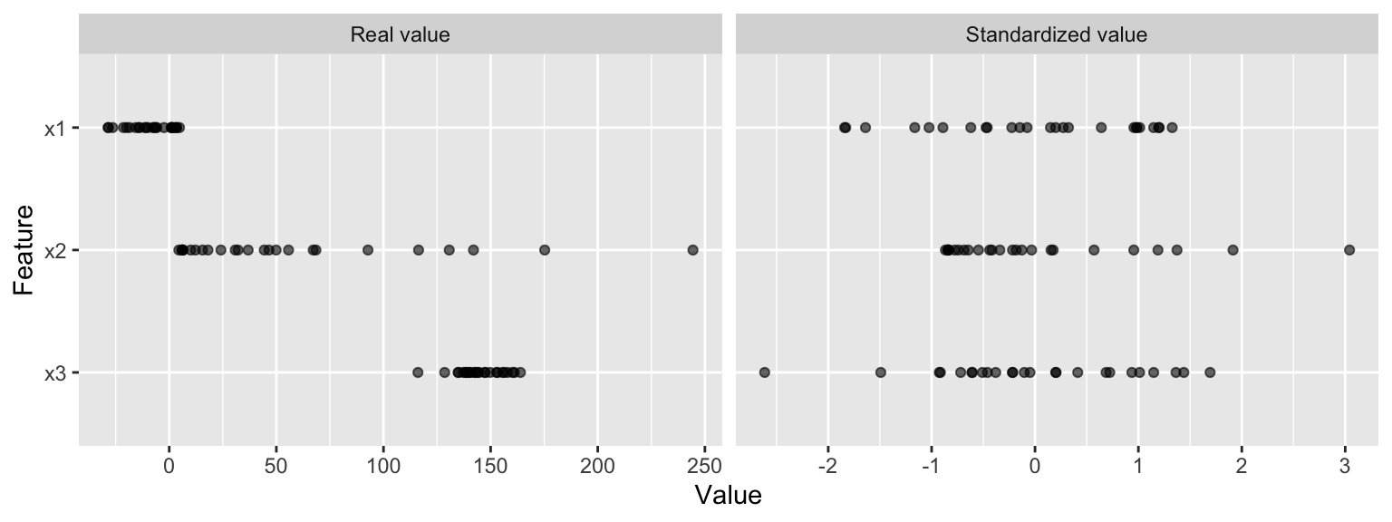
Figure 8.1: Standardizing features allows all features to be compared on a common value scale regardless of their real value differences.
We can standardize our numeric features in one of two ways – note that step_normalize() is just a wrapper that combines step_center() and step_scale().
# option 1
std <- ames_recipe %>%
   step_center(all_numeric_predictors()) %>%
   step_scale(all_numeric_predictors())

# option 2
std <- ames_recipe %>%
   step_normalize(all_numeric_predictors())
Note how we did not specify an individual variable within our step_xxx() functions. You can certain do that if you wanted to. For example, if you just wanted to standardize the Gr_Liv_Area and Year_Built feature you could with:
However, instead we used selectors to apply this recipe step to all the numeric features at once using all_nominal_predictors(). The selector functions can be combined to select intersections of variables just like we learned several weeks ago with the dplyr::select() function.
The result of the above code is not to actually apply the feature engineering steps but, rather, to create an object that holds the feature engineering logic (or recipe) to be applied later on.
8.4.2 Normalizing
Parametric models that have distributional assumptions can benefit from minimizing the skewness of numeric features. For instance, ordinary linear regression models assume that the prediction errors are normally distributed. However, sometimes when certain features or even the response variable has heavy tails (i.e., outliers) or is skewed in one direction or the other, this normality assumption will likely not hold.
There are two main approaches to help correct for skewed feature variables:
Option 1: normalize with a log transformation. This will transform most right skewed distributions to be approximately normal.
However, if your feature(s) have negative values or zeros then a log transformation will produce NaNs and -Infs, respectively (you cannot take the logarithm of a negative number). If the non positive response values are small (say between -0.99 and 0) then you can apply a small offset such as in log1p() which adds 1 to the value prior to applying a log transformation (you can do the same within step_log() by using the offset argument).
If your data consists of values \(\leq -1\), use the Yeo-Johnson transformation mentioned next.
Option 2: use a Box Cox transformation. A Box Cox transformation is more flexible than (but also includes as a special case) the log transformation and will find an appropriate transformation from a family of power transforms that will transform the variable as close as possible to a normal distribution (Box and Cox 1964; Carroll and Ruppert 1981). At the core of the Box Cox transformation is an exponent, lambda (\(\lambda\)), which varies from -5 to 5. All values of \(\lambda\) are considered and the optimal value for the given data is estimated from the training data; The “optimal value” is the one which results in the best transformation to an approximate normal distribution. The transformation of the response \(Y\) has the form:
\[ \begin{equation} y(\lambda) = \begin{cases} \frac{Y^\lambda-1}{\lambda}, & \text{if}\ \lambda \neq 0 \\ \log\left(Y\right), & \text{if}\ \lambda = 0. \end{cases} \end{equation} \]
If your response has negative values, the Yeo-Johnson transformation is very similar to the Box-Cox but does not require the input variables to be strictly positive.
We can normalize our numeric predictor variables with step_YeoJohnson():
8.4.3 Knowledge check
Using the boston_train data, fill in the blanks to
create a recipe that…
-
Models
cmedvas a function of all predictors, - standardizes all numeric features,
- Normalizes all all numeric features with a Yeo-Johnson transformation
boston_recipe <- recipe(_______ ~ _______, data = boston_train) %>%
   step_______(___________) %>%
   step_______(___________)
8.5 Categorical features
Most models require that the predictors take numeric form. There are exceptions; for example, some tree-based models naturally handle numeric or categorical features. However, even tree-based models can benefit from pre-processing categorical features. The following sections will discuss a few of the more common approaches to engineer categorical features.
8.5.1 One-hot & dummy encoding
There are many ways to recode categorical variables as numeric. The most common is referred to as one-hot encoding, where we transpose our categorical variables so that each level of the feature is represented as a boolean value. For example, one-hot encoding the left data frame in the below figure results in X being converted into three columns, one for each level. This is called less than full rank encoding . However, this creates perfect collinearity which causes problems with some predictive modeling algorithms (e.g., ordinary linear regression and neural networks). Alternatively, we can create a full-rank encoding by dropping one of the levels (level c has been dropped). This is referred to as dummy encoding.
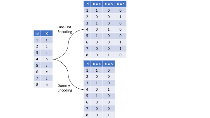
Figure 8.2: Eight observations containing a categorical feature X and the difference in how one-hot and dummy encoding transforms this feature.
We can use step_dummy() to add a one-hot or dummy encoding to our recipe:
# one-hot encode
ohe <- ames_recipe %>%
  step_dummy(all_nominal(), one_hot = TRUE)

# dummy encode
de <- ames_recipe %>%
  step_dummy(all_nominal(), one_hot = FALSE)
Recall our lesson on applying an ordinary least squares regression model to a categorical feature. Behind the scenes R was automatically dummy encoding our categorical feature; however, many (dare I say most) algorithms will not automatically do that for us.
8.5.2 Ordinal encoding
If a categorical feature is naturally ordered then numerically encoding the feature based on its order is a natural choice (most commonly referred to as ordinal encoding). For example, the various quality features in the Ames housing data are ordinal in nature (ranging from Very_Poor to Very_Excellent).
ames_train %>% select(matches('Qual$|QC$|_Cond$'))
## # A tibble: 2,051 × 11
##    Overall_Qual  Overall_Cond Exter_Qual Exter_Cond Bsmt_Qual Bsmt_Cond
##    <chr>         <chr>        <chr>      <chr>      <chr>     <chr>
##  1 Very_Good     Average      Good       Typical    Good      Good
##  2 Above_Average Average      Good       Typical    Good      Typical
##  3 Below_Average Average      Typical    Typical    Good      Typical
##  4 Very_Good     Average      Good       Typical    Good      Typical
##  5 Above_Average Good         Typical    Typical    Typical   Good
##  6 Good          Average      Good       Typical    Good      Typical
##  7 Above_Average Average      Typical    Typical    Good      Typical
##  8 Average       Average      Typical    Typical    Typical   Typical
##  9 Average       Good         Typical    Typical    Fair      Typical
## 10 Below_Average Average      Typical    Typical    Typical   Typical
## # ℹ 2,041 more rows
## # ℹ 5 more variables: Heating_QC <chr>, Kitchen_Qual <chr>,
## #   Garage_Qual <chr>, Garage_Cond <chr>, Pool_QC <chr>
Ordinal encoding these features provides a natural and intuitive interpretation and can logically be applied to all models.
If your features are already ordered factors then you can simply apply step_ordinalscore() to ordinal encode:
However, if we look at our quality features we see they are characters instead of factors and their levels are not ordered. Moreover, some have a unique value that represents that feature doesn’t exist in the house (i.e. No_Basement).
ames_train %>% pull(Bsmt_Qual) %>% unique()
## [1] "Good"        "Typical"     "Fair"        "Excellent"
## [5] "No_Basement" "Poor"
So in this case we’re going to apply several feature engineering steps to:
- convert quality features to factors with specified levels,
- convert any missed levels (i.e. No_Basement, No_Pool) to “None”,
- convert factor level to integer value (‘Very_Poor’ = 1, ‘Poor’ = 2, …, ‘Excellent’ = 10, ‘Very_Excellent’ = 11)
# specify levels in order
lvls <- c("Very_Poor", "Poor", "Fair", "Below_Average", "Average", "Typical",
          "Above_Average", "Good", "Very_Good", "Excellent", "Very_Excellent")

# apply ordinal encoding to quality features
ord_lbl <- ames_recipe %>%
   # 1. convert quality features to factors with specified levels
   step_string2factor(matches('Qual$|QC$|_Cond$'), levels = lvls, ordered = TRUE) %>%
   # 2. convert any missed levels (i.e. No_Basement, No_Pool) to "None"
   step_unknown(matches('Qual$|QC$|_Cond$'), new_level = "None") %>%
   # 3. convert factor level to integer value
   step_ordinalscore(matches('Qual$|QC$|_Cond$'))
Did this work, let’s take a look. If we want to apply a recipe to a data set we can apply:
prep: estimate feature engineering parameters based on training data.bake: apply the prepped recipe to new, or the existing (new_data = NULL) data.
We can see that our quality variables are now ordinal encoded.
baked_recipe <- ord_lbl %>%
   prep(strings_as_factor = FALSE) %>%
   bake(new_data = NULL)

baked_recipe %>% select(matches('Qual$|QC$|_Cond$'))
## # A tibble: 2,051 × 11
##    Overall_Qual Overall_Cond Exter_Qual Exter_Cond Bsmt_Qual Bsmt_Cond
##           <int>        <int>      <int>      <int>     <int>     <int>
##  1            9            5          8          6         8         8
##  2            7            5          8          6         8         6
##  3            4            5          6          6         8         6
##  4            9            5          8          6         8         6
##  5            7            8          6          6         6         8
##  6            8            5          8          6         8         6
##  7            7            5          6          6         8         6
##  8            5            5          6          6         6         6
##  9            5            8          6          6         3         6
## 10            4            5          6          6         6         6
## # ℹ 2,041 more rows
## # ℹ 5 more variables: Heating_QC <int>, Kitchen_Qual <int>,
## #   Garage_Qual <int>, Garage_Cond <int>, Pool_QC <int>
And if we want to see how the numeric values are mapped to the original data we can. Here, I just focus on the original Overall_Qual values and how they compare to the encoded values.
encoded_Overall_Qual <- baked_recipe %>%
   select(Overall_Qual) %>%
   rename(encoded_Overall_Qual = Overall_Qual)

ames_train %>%
   select(Overall_Qual) %>%
   bind_cols(encoded_Overall_Qual) %>%
   count(Overall_Qual, encoded_Overall_Qual)
## # A tibble: 10 × 3
##    Overall_Qual   encoded_Overall_Qual     n
##    <chr>                         <int> <int>
##  1 Above_Average                     7   509
##  2 Average                           5   587
##  3 Below_Average                     4   168
##  4 Excellent                        10    65
##  5 Fair                              3    30
##  6 Good                              8   419
##  7 Poor                              2     9
##  8 Very_Excellent                   11    26
##  9 Very_Good                         9   235
## 10 Very_Poor                         1     3
8.5.3 Lumping
Sometimes features will contain levels that have very few observations. For example, there are 28 unique neighborhoods represented in the Ames housing data but several of them only have a few observations.
## # A tibble: 28 × 2
##    Neighborhood            n
##    <chr>               <int>
##  1 Green_Hills             1
##  2 Landmark                1
##  3 Greens                  6
##  4 Blueste                 8
##  5 Northpark_Villa        16
##  6 Veenker                18
##  7 Briardale              20
##  8 Bloomington_Heights    22
##  9 Meadow_Village         26
## 10 Clear_Creek            29
## # ℹ 18 more rows
Sometimes we can benefit from collapsing, or “lumping” these into a lesser number of categories. In the above examples, we may want to collapse all levels that are observed in less than 1% of the training sample into an “other” category. We can use step_other() to do so. However, lumping should be used sparingly as there is often a loss in model performance (Kuhn and Johnson 2013).
Tree-based models often perform exceptionally well with high cardinality features and are not as impacted by levels with small representation.
The following lumps all neighborhoods that represent less than 1% of observations into an “other” category.
8.5.4 Knowledge check
Using the Ames data, fill in the blanks to
-
ordinal encode the
Overall_Condvariable and -
lump all
Neighborhoods that represent less than 1% of observations into an “other” category.
# specify levels in order
lvls <- c("Very_Poor", "Poor", "Fair", "Below_Average", "Average",
          "Above_Average", "Good", "Very_Good", "Excellent")

cat_encode <- ames_recipe %>%
   # 1. convert quality features to factors with specified levels
   step_string2factor(_______, levels = ___, ordered = ____) %>%
   # 2. convert factor level to integer value
   step_ordinalscore(______) %>%
   # 3. lump novel neighborhood levels
   step_other(______, threshold = ____, other = "other")
8.6 Fit a model with a recipe
Alright, so we know how to do a little feature engineering, now let’s put it to use. Recall that we are using the ames.csv data rather than the AmesHousing::make_ames() data. Because of this if we were to try train a multiple linear regression model on all the predictors we would get an error when applying that model to unseen data (i.e. ames_test).
This is because there are some rare levels in some of the categorical features.
linear_reg() %>%
   fit(Sale_Price ~ ., data = ames_train) %>%
   predict(ames_test) %>%
   bind_cols(ames_test) %>%
   rmse(truth = Sale_Price, estimate = .pred)
## Error in model.frame.default(Terms, newdata, na.action = na.action, xlev = object$xlevels): factor Roof_Matl has new levels Metal, Roll
If we remove all the categorical features with rare levels we can train a model and apply it to our test data.
Note that our result differs from the last lesson because we are
using ames.csv rather than the
AmesHousing::make_ames() data and there are some subtle
differences between those data sets.
trbl_vars <- c("MS_SubClass", "Condition_2", "Exterior_1st",
               "Exterior_2nd", "Misc_Feature", "Roof_Matl",
               "Electrical", "Sale_Type")
ames_smaller_train <- ames_train %>%
   select(-trbl_vars)

linear_reg() %>%
   fit(Sale_Price ~ ., data = ames_smaller_train) %>%
   predict(ames_test) %>%
   bind_cols(ames_test) %>%
   rmse(truth = Sale_Price, estimate = .pred)
## # A tibble: 1 × 3
##   .metric .estimator .estimate
##   <chr>   <chr>          <dbl>
## 1 rmse    standard      31296.
Unfortunately, we dropped the troublesome categorical features which may actually have some useful information in them. Also, we may be able to improve performance by applying other feature engineering steps. Let’s combine some feature engineering tasks into one recipe and then train a model with it.
final_recipe <- recipe(Sale_Price ~ ., data = ames_train) %>%
   step_nzv(all_predictors(), unique_cut = 10) %>%
   step_YeoJohnson(all_numeric_predictors()) %>%
   step_normalize(all_numeric_predictors()) %>%
   step_string2factor(matches('Qual$|QC$|_Cond$'), levels = lvls, ordered = TRUE) %>%
   step_unknown(matches('Qual$|QC$|_Cond$'), new_level = "None") %>%
   step_integer(matches('Qual$|QC$|_Cond$')) %>%
   step_other(all_nominal_predictors(), threshold = 0.01, other = "other")
We will want to use our recipe across several steps as we train and test our model. We will:
Process the recipe using the training set: This involves any estimation or calculations based on the training set. For our recipe, the training set will be used to determine which predictors will have zero-variance in the training set, and should be slated for removal, what the mean and scale is in order to standardize the numeric features, etc.
Apply the recipe to the training set: We create the final predictor set on the training set.
Apply the recipe to the test set: We create the final predictor set on the test set. Nothing is recomputed and no information from the test set is used here; the feature engineering statistics computed from the training set are applied to the test set.
To simplify this process, we can use a model workflow, which pairs a model and recipe together. This is a straightforward approach because different recipes are often needed for different models, so when a model and recipe are bundled, it becomes easier to train and test workflows. We’ll use the workflows package from tidymodels to bundle our model with our recipe (ames_recipe).
mlr_wflow <- workflow() %>%
  add_model(linear_reg()) %>%
  add_recipe(final_recipe)

mlr_wflow
## ══ Workflow ═══════════════════════════════════════════════════════════
## Preprocessor: Recipe
## Model: linear_reg()
##
## ── Preprocessor ───────────────────────────────────────────────────────
## 7 Recipe Steps
##
## • step_nzv()
## • step_YeoJohnson()
## • step_normalize()
## • step_string2factor()
## • step_unknown()
## • step_integer()
## • step_other()
##
## ── Model ──────────────────────────────────────────────────────────────
## Linear Regression Model Specification (regression)
##
## Computational engine: lm
Now, there is a single function that can be used to prepare the recipe and train the model from the resulting predictors:
The rf_fit object has the finalized recipe and fitted model objects inside. You may want to extract the model or recipe objects from the workflow. To do this, you can use the helper functions extract_fit_parsnip() and extract_recipe().
mlr_fit %>%
   extract_fit_parsnip() %>%
   tidy()
## # A tibble: 163 × 5
##    term                            estimate std.error statistic p.value
##    <chr>                              <dbl>     <dbl>     <dbl>   <dbl>
##  1 (Intercept)                      168020.    29181.    5.76   9.92e-9
##  2 MS_SubClassOne_and_Half_Story_…    -460.    26648.   -0.0173 9.86e-1
##  3 MS_SubClassOne_Story_1945_and_…   10808.    26368.    0.410  6.82e-1
##  4 MS_SubClassOne_Story_1946_and_…    2180.    25692.    0.0849 9.32e-1
##  5 MS_SubClassOne_Story_PUD_1946_…  -18599.    28321.   -0.657  5.11e-1
##  6 MS_SubClassSplit_Foyer             7735.    27007.    0.286  7.75e-1
##  7 MS_SubClassSplit_or_Multilevel     9553.    29836.    0.320  7.49e-1
##  8 MS_SubClassTwo_Family_conversi…    7485.     6934.    1.08   2.81e-1
##  9 MS_SubClassTwo_Story_1945_and_…    9382.    26359.    0.356  7.22e-1
## 10 MS_SubClassTwo_Story_1946_and_…   -1677.    25542.   -0.0657 9.48e-1
## # ℹ 153 more rows
Just as in the last lesson, we can make predictions with our fit model object and evaluate the model performance. Here, we compute the RMSE on our ames_test data and we see we have a better performance than the previous model that had no feature engineering steps.
mlr_fit %>%
   predict(ames_test) %>%
   bind_cols(ames_test %>% select(Sale_Price)) %>%
   rmse(truth = Sale_Price, estimate = .pred)
## # A tibble: 1 × 3
##   .metric .estimator .estimate
##   <chr>   <chr>          <dbl>
## 1 rmse    standard      29729.
8.6.1 Knowledge check
Using the boston_train data, fill in the blanks to train a model with the given recipe…
-
The recipe should model
cmedvas a function of all predictors, - standardizes all numeric features,
- Normalizes all all numeric features with a Yeo-Johnson transformation
# 1. Create recipe
boston_recipe <- recipe(_____ ~ _____, data = boston_train) %>%
  step______(_____) %>%
  step______(_____)

# 2. Create a workflow object
mlr_wflow <- workflow() %>%
  add_model(_____) %>%
  add_recipe(_____)

# 3. Fit and evaluate our model like we did before
mlr_fit <- mlr_wflow %>%
   fit(data = boston_train)

mlr_fit %>%
   predict(boston_test) %>%
   bind_cols(boston_test %>% select(cmedv)) %>%
   rmse(truth = cmedv, estimate = .pred)
8.7 Exercises
-
Identify three new feature engineering steps that are provided by recipes. Why would these feature engineering steps be applicable to the Ames data?
-
Using the
boston.csvdata, create a multiple linear regression model using all predictors in their current state. Now apply feature engineering steps to standardize and normalize the numeric features prior to modeling. Does the model performance improve? -
Using the
AmesHousing::make_ames()rebuild the model we created in this section. However, rather than remove the trouble variables, apply a feature engineering step to lump novel levels together so that you can use those variables as predictors. Does the model performance improve?