17 Lesson 6a: Decision Trees

Tree-based models are a class of nonparametric algorithms that work by partitioning the feature space into a number of smaller (non-overlapping) regions with similar response values using a set of splitting rules. Predictions are obtained by fitting a simpler model (e.g., a constant like the average response value) in each region. Such divide-and-conquer methods can produce simple rules that are easy to interpret and visualize with tree diagrams. As we’ll see, decision trees offer many benefits; however, they typically lack in predictive performance compared to more complex algorithms like neural networks and MARS. However, future modules will discuss powerful ensemble algorithms—like random forests and gradient boosting machines—which are constructed by combining together many decision trees in a clever way. This module will provide you with a strong foundation in decision trees.

17.1 Learning objectives

By the end of this module you will know:

• How decision tree models partition data and how the depth of a tree impacts performance.
• Train, fit, tune and assess decision tree models.
• Identify important features and visualize their influence on the response.

17.2 Prerequisites

# Helper packages
library(tidyverse)   # for data wrangling & plotting

# Modeling packages
library(tidymodels) 

# Model interpretability packages
library(vip)         # for variable importance
library(pdp)         # for variable relationships

set.seed(123)
ames <- AmesHousing::make_ames()
split  <- initial_split(ames, prop = 0.7, strata = "Sale_Price")
ames_train  <- training(split)
ames_test   <- testing(split)

17.3 Structure

There are many methodologies for constructing decision trees but the most well-known is the classification and regression tree (CART) algorithm proposed in Breiman (1984).⁶ A basic decision tree partitions the training data into homogeneous subgroups (i.e., groups with similar response values) and then fits a simple constant in each subgroup (e.g., the mean of the within group response values for regression). The subgroups (also called nodes) are formed recursively using binary partitions formed by asking simple yes-or-no questions about each feature (e.g., is age < 18?). This is done a number of times until a suitable stopping criteria is satisfied (e.g., a maximum depth of the tree is reached). After all the partitioning has been done, the model predicts the output based on (1) the average response values for all observations that fall in that subgroup (regression problem), or (2) the class that has majority representation (classification problem). For classification, predicted probabilities can be obtained using the proportion of each class within the subgroup.

What results is an inverted tree-like structure such as that in the below figure. In essence, our tree is a set of rules that allows us to make predictions by asking simple yes-or-no questions about each feature. For example, if the customer is loyal, has household income greater than $150,000, and is shopping in a store, the exemplar tree diagram below would predict that the customer will redeem a coupon.

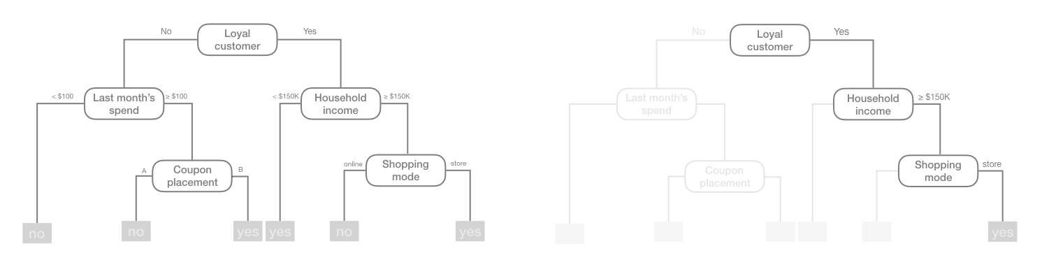
Figure 17.1: Exemplar decision tree predicting whether or not a customer will redeem a coupon (yes or no) based on the customer’s loyalty, household income, last month’s spend, coupon placement, and shopping mode.

We refer to the first subgroup at the top of the tree as the root node (this node contains all of the training data). The root node shows the first feature that best splits the data into two groups. The final subgroups at the bottom of the tree are called the terminal nodes or leaves. These terminal nodes represent predicted values once you have traversed a particular path down the tree. Every subgroup in between is referred to as an internal node. The connections between nodes are called branches.

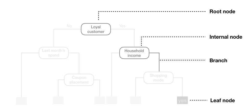
Figure 17.2: Terminology of a decision tree.

17.4 Partitioning

As illustrated above, CART uses binary recursive partitioning (it’s recursive because each split or rule depends on the the splits above it). The objective at each node is to find the “best” feature (\(x_i\)) to partition the remaining data into one of two regions (\(R_1\) and \(R_2\)) such that the overall error between the actual response (\(y_i\)) and the predicted constant (\(c_i\)) is minimized. For regression problems, the objective function to minimize is the total SSE as defined in the following equation:

\[\begin{equation} SSE = \sum_{i \in R_1}\left(y_i - c_1\right)^2 + \sum_{i \in R_2}\left(y_i - c_2\right)^2 \end{equation}\]

For classification problems, the partitioning is usually made to maximize the reduction in cross-entropy or the Gini index.⁷

In both regression and classification trees, the objective of partitioning is to minimize dissimilarity in the terminal nodes. However, we suggest Therneau, Atkinson, et al. (1997) for a more thorough discussion regarding binary recursive partitioning.

Having found the best feature/split combination, the data are partitioned into two regions and the splitting process is repeated on each of the two regions (hence the name binary recursive partitioning). This process is continued until a suitable stopping criterion is reached (e.g., a maximum depth is reached or the tree becomes “too complex”).

It’s important to note that a single feature can be used multiple times in a tree. For example, say we have data generated from a simple \(\sin\) function with Gaussian noise: \(Y_i \stackrel{iid}{\sim} N\left(\sin\left(X_i\right), \sigma^2\right)\), for \(i = 1, 2, \dots, 500\). A regression tree built with a single root node (often referred to as a decision stump) leads to a split occurring at \(x = 3.1\).

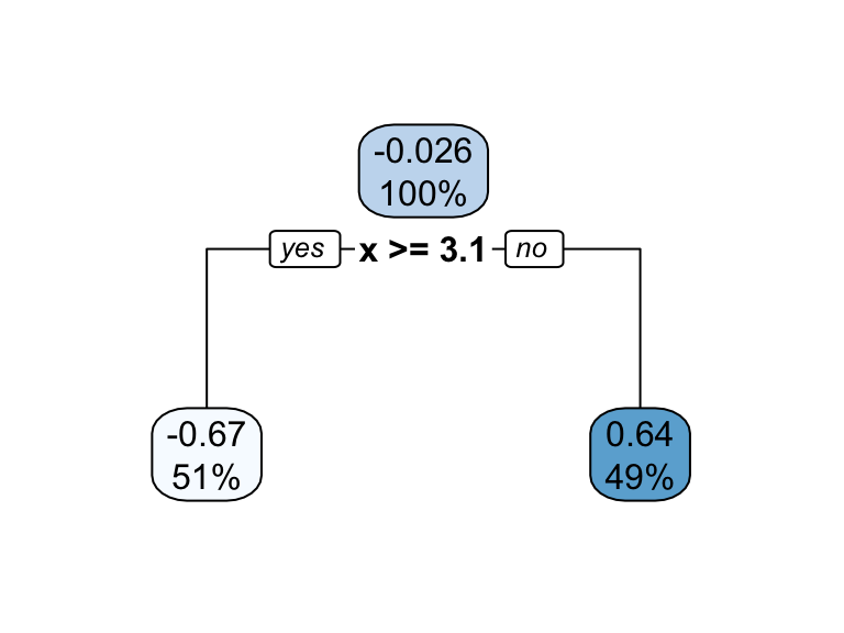
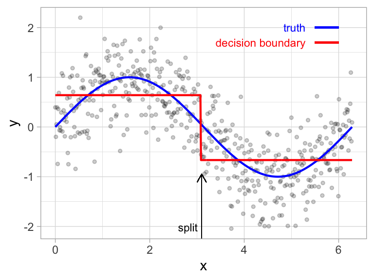
Figure 17.3: Decision tree illustrating the single split on feature x (left). The resulting decision boundary illustrates the predicted value when x < 3.1 (0.64), and when x > 3.1 (-0.67) (right).

If we build a deeper tree, we’ll continue to split on the same feature (\(x\)) as illustrated below. This is because \(x\) is the only feature available to split on so it will continue finding the optimal splits along this feature’s values until a pre-determined stopping criteria is reached.

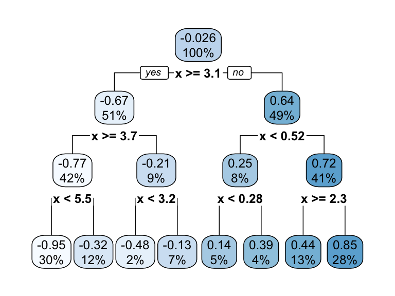
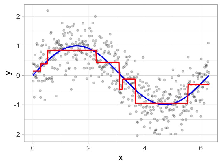
Figure 17.4: Decision tree illustrating with depth = 3, resulting in 7 decision splits along values of feature x and 8 prediction regions (left). The resulting decision boundary (right).

However, even when many features are available, a single feature may still dominate if it continues to provide the best split after each successive partition. For example, a decision tree applied to the iris data set (R. A. Fisher 1936) where the species of the flower (setosa, versicolor, and virginica) is predicted based on two features (sepal width and sepal length) results in an optimal decision tree with two splits on each feature. Also, note how the decision boundary in a classification problem results in rectangular regions enclosing the observations. The predicted value is the response class with the greatest proportion within the enclosed region.

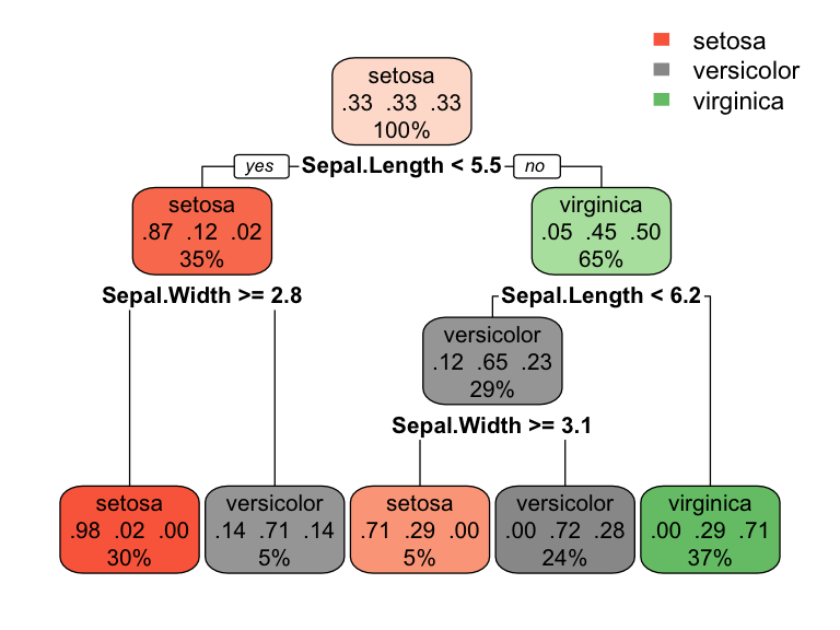
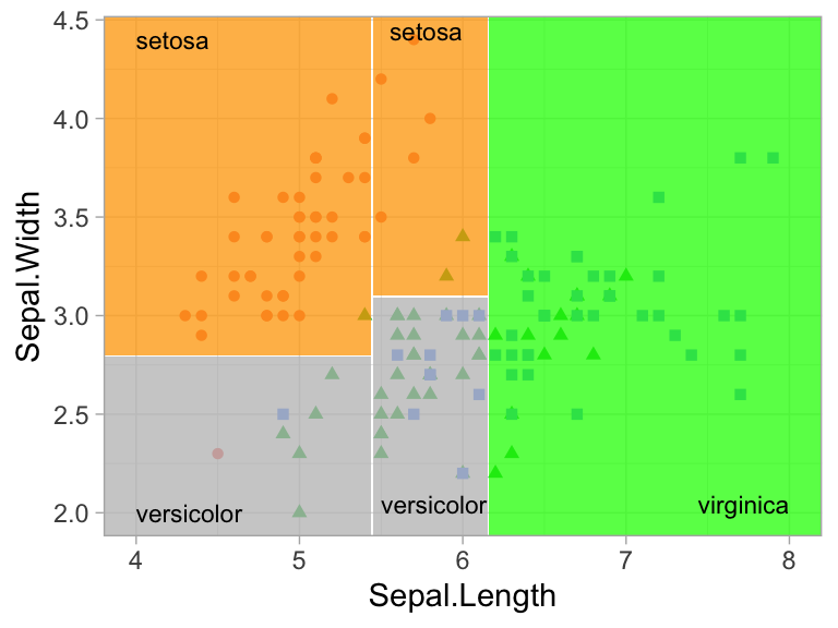
Figure 17.5: Decision tree for the iris classification problem (left). The decision boundary results in rectangular regions that enclose the observations. The class with the highest proportion in each region is the predicted value (right).

17.5 How deep?

This leads to an important question: how deep (i.e., complex) should we make the tree? If we grow an overly complex tree as in the below figure, we tend to overfit to our training data resulting in poor generalization performance.

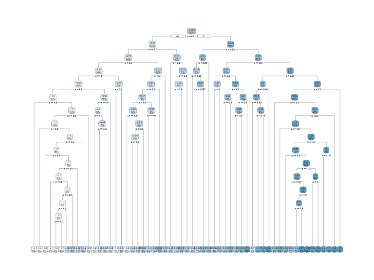
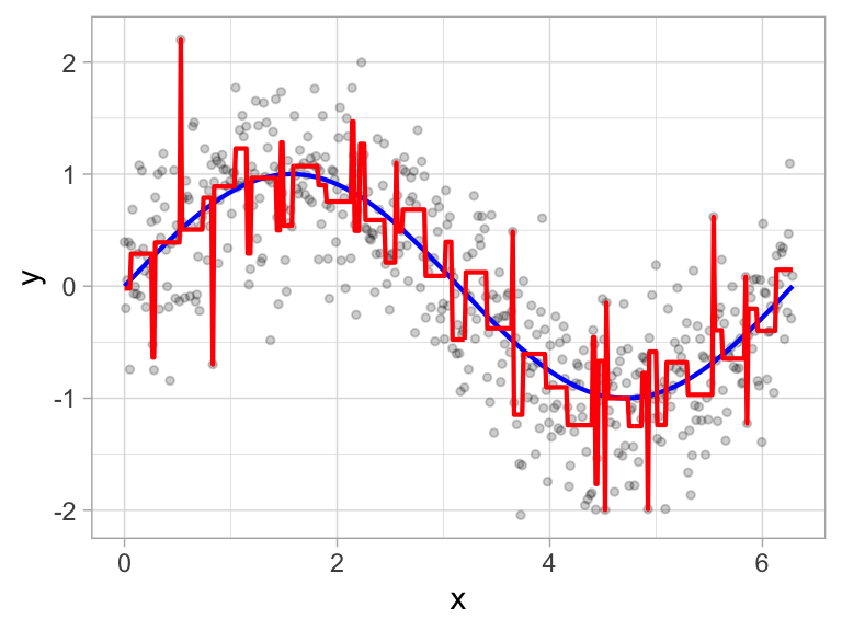
Figure 17.6: Overfit decision tree with 56 splits.

Consequently, there is a balance to be achieved in the depth and complexity of the tree to optimize predictive performance on future unseen data. To find this balance, we have two primary approaches: (1) early stopping and (2) pruning.

17.5.1 Early stopping

Early stopping explicitly restricts the growth of the tree. There are several ways we can restrict tree growth but two of the most common approaches are to restrict the tree depth to a certain level or to restrict the minimum number of observations allowed in any terminal node. When limiting tree depth we stop splitting after a certain depth (e.g., only grow a tree that has a depth of 5 levels). The shallower the tree the less variance we have in our predictions; however, at some point we can start to inject too much bias as shallow trees (e.g., stumps) are not able to capture interactions and complex patterns in our data.

When restricting minimum terminal node size (e.g., leaf nodes must contain at least 10 observations for predictions) we are deciding to not split intermediate nodes which contain too few data points. At the far end of the spectrum, a terminal node’s size of one allows for a single observation to be captured in the leaf node and used as a prediction (in this case, we’re interpolating the training data). This results in high variance and poor generalizability. On the other hand, large values restrict further splits therefore reducing variance.

These two approaches can be implemented independently of one another; however, they do have interaction effects as illustrated below.

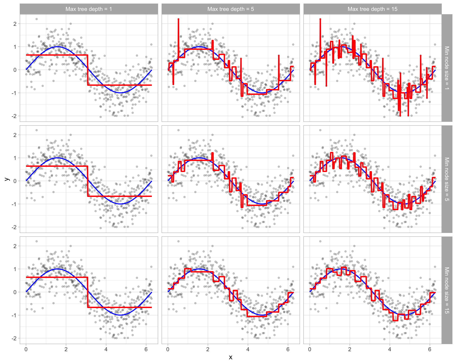
Figure 17.7: Illustration of how early stopping affects the decision boundary of a regression decision tree. The columns illustrate how tree depth impacts the decision boundary and the rows illustrate how the minimum number of observations in the terminal node influences the decision boundary.

17.5.2 Pruning

An alternative to explicitly specifying the depth of a decision tree is to grow a very large, complex tree and then prune it back to find an optimal subtree. We find the optimal subtree by using a cost complexity parameter (\(\alpha\)) that penalizes our objective function for the number of terminal nodes of the tree (\(T\)) as in the following equation.

\[\begin{equation} \texttt{minimize} \left\{ SSE + \alpha \vert T \vert \right\} \end{equation}\]

For a given value of \(\alpha\) we find the smallest pruned tree that has the lowest penalized error. You may recognize the close association to the lasso penalty discussed in the regularized regression lesson. As with the regularization methods, smaller penalties tend to produce more complex models, which result in larger trees. Whereas larger penalties result in much smaller trees. Consequently, as a tree grows larger, the reduction in the SSE must be greater than the cost complexity penalty. Typically, we evaluate multiple models across a spectrum of \(\alpha\) and use CV to identify the optimal value and, therefore, the optimal subtree that generalizes best to unseen data.

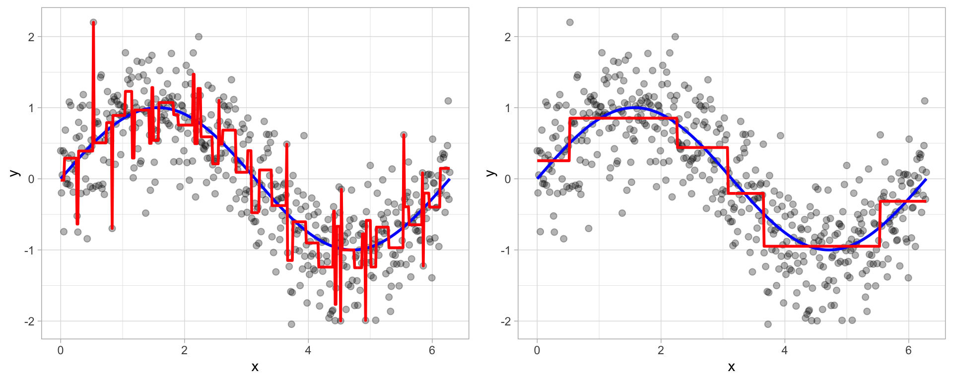
Figure 17.8: To prune a tree, we grow an overly complex tree (left) and then use a cost complexity parameter to identify the optimal subtree (right).

17.6 Fitting a decision tree

17.6.1 Fitting a basic model

To illustrate some of the concepts we’ve mentioned we’ll start by implementing models using just the Gr_Liv_Area and Year_Built features in our Ames housing data.

In R we use the decision_tree() model and we’ll use the rpart package as our model engine. In this example we will not set a specific depth of our tree; rather, rpart automatically builds a fully deep tree and then prunes it to attempt to find an optimal tree depth.

# Step 1: create decision tree model object
dt_mod <- decision_tree(mode = "regression") %>% set_engine("rpart")

# Step 2: create model recipe
model_recipe <- recipe(
    Sale_Price ~ Gr_Liv_Area + Year_Built, 
    data = ames_train
  )
  
# Step 3: fit model workflow
dt_fit <- workflow() %>%
  add_recipe(model_recipe) %>%
  add_model(dt_mod) %>%
  fit(data = ames_train)

# Step 4: results
dt_fit
## ══ Workflow [trained] ══════════════════════
## Preprocessor: Recipe
## Model: decision_tree()
## 
## ── Preprocessor ────────────────────────────
## 0 Recipe Steps
## 
## ── Model ───────────────────────────────────
## n= 2049 
## 
## node), split, n, deviance, yval
##       * denotes terminal node
## 
##  1) root 2049 1.321981e+13 180922.6  
##    2) Year_Built< 1985.5 1228 2.698241e+12 141467.4  
##      4) Gr_Liv_Area< 1486 840 7.763942e+11 125692.6  
##        8) Year_Built< 1952.5 317 2.687202e+11 107761.5 *
##        9) Year_Built>=1952.5 523 3.439725e+11 136561.0 *
##      5) Gr_Liv_Area>=1486 388 1.260276e+12 175619.2  
##       10) Gr_Liv_Area< 2663.5 372 8.913502e+11 170223.5 *
##       11) Gr_Liv_Area>=2663.5 16 1.062939e+11 301068.8 *
##    3) Year_Built>=1985.5 821 5.750622e+12 239937.1  
##      6) Gr_Liv_Area< 1963 622 1.813069e+12 211699.5  
##       12) Gr_Liv_Area< 1501.5 285 3.483774e+11 182098.8 *
##       13) Gr_Liv_Area>=1501.5 337 1.003788e+12 236732.8  
##         26) Year_Built< 2004.5 198 3.906393e+11 217241.1 *
##         27) Year_Built>=2004.5 139 4.307663e+11 264498.0 *
##      7) Gr_Liv_Area>=1963 199 1.891416e+12 328197.2  
##       14) Gr_Liv_Area< 2390.5 107 5.903157e+11 290924.0  
##         28) Year_Built< 2004.5 69 1.168804e+11 253975.7 *
##         29) Year_Built>=2004.5 38 2.081946e+11 358014.5 *
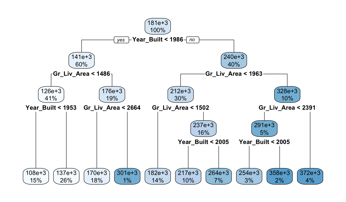
##       15) Gr_Liv_Area>=2390.5 92 9.795556e+11 371547.5 *

We can use rpart.plot() to plot our tree. This is only useful if we have a relatively small tree to visualize; however, most trees we will build will be far too large to attempt to visualize. In this case, we see that the root node (first node) splits our data based on (Year_Built). For those observations where the home is built after 1985 we follow the right half of the decision tree and for those where the home is built in or prior to 1985 we follow the left half of the decision tree.

rpart.plot::rpart.plot(dt_fit$fit$fit$fit)

However, to understand how our model is performing we want to perform cross validation. We see that this single decision tree is not performing spectacularly well with the average RMSE across our 5 folds equaling just under $50K.

# create resampling procedure
set.seed(13)
kfold <- vfold_cv(ames_train, v = 5)

# train model
results <- fit_resamples(dt_mod, model_recipe, kfold)

# model results
collect_metrics(results)
## # A tibble: 2 × 6
##   .metric .estimator      mean     n std_err
##   <chr>   <chr>          <dbl> <int>   <dbl>
## 1 rmse    standard   47178.        5 1.19e+3
## 2 rsq     standard       0.655     5 1.29e-2
## # ℹ 1 more variable: .config <chr>

17.6.2 Fitting a full model

Next, lets go ahead and fit a full model to include all Ames housing features. We do not need to one-hot encode our features as rpart will naturally handle categorical features. By including all features we see some improvement in our model performance as our average cross validated RMSE is now in the low $40K range.

# create model recipe with all features
full_model_recipe <- recipe(
    Sale_Price ~ ., 
    data = ames_train
  )

# train model
results <- fit_resamples(dt_mod, full_model_recipe, kfold)

# model results
collect_metrics(results)
## # A tibble: 2 × 6
##   .metric .estimator      mean     n std_err
##   <chr>   <chr>          <dbl> <int>   <dbl>
## 1 rmse    standard   40510.        5 1.69e+3
## 2 rsq     standard       0.745     5 1.48e-2
## # ℹ 1 more variable: .config <chr>

17.6.3 Knowledge check

Using the boston.csv dataset:

1. Apply a default decision tree model where cmedv is the response variable and rm and lstat are the two predictor variables.
   • Assess the resulting tree and explain the first decision node.
   • Pick a branch and explain the decision nodes as you traverse down the branch.
2. Apply a decision tree model that uses all possible predictor variables.
   • Assess the resulting tree and explain the first decision node.
   • Pick a branch and explain the decision nodes as you traverse down the branch.
3. Use a 5-fold cross validation procedure to compare the model in #1 to the model in #2. Which model performs best?

17.7 Tuning

As previously mentioned, the tree depth is the primary factor that impacts performance. We can control tree depth via a few different parameters:

1. Max depth: we can explicitly state the maximum depth a tree can be grown.
2. Minimum observations for a split: The minimum number of samples required to split an internal node. This limits a tree from continuing to grow as the number of observations in a give node becomes smaller.
3. Cost complexity parameter: acts as a regularization mechanism by penalizing the objective function.

There is not one best approach to use and often different combinations of these parameter settings improves model performance. The following will demonstrate a small grid search across 3 different values for each of these parameters (\(3^3 = 27\) total setting combinations).

# create model object with tuning options
dt_mod <- decision_tree(
  mode = "regression",
  cost_complexity = tune(),
  tree_depth = tune(),
  min_n = tune()
 ) %>% 
  set_engine("rpart")

# create the hyperparameter grid
hyper_grid <- grid_regular(
  cost_complexity(), 
  tree_depth(),
  min_n()
 )

# hyperparameter value combinations to be assessed
hyper_grid
## # A tibble: 27 × 3
##    cost_complexity tree_depth min_n
##              <dbl>      <int> <int>
##  1    0.0000000001          1     2
##  2    0.00000316            1     2
##  3    0.1                   1     2
##  4    0.0000000001          8     2
##  5    0.00000316            8     2
##  6    0.1                   8     2
##  7    0.0000000001         15     2
##  8    0.00000316           15     2
##  9    0.1                  15     2
## 10    0.0000000001          1    21
## # ℹ 17 more rows

We can now perform our grid search using tune_grid(). We see the optimal model decreases our average CV RMSE into the mid $30K range.

It is common to run additional grid searches after the first grid search. These additional grid searches uses the first grid search to find parameter values that perform well and then continue to analyze additional ranges around these values.

# train our model across the hyper parameter grid
set.seed(123)
results <- tune_grid(dt_mod, full_model_recipe, resamples = kfold, grid = hyper_grid)

# get best results
show_best(results, metric = "rmse", n = 10)
## # A tibble: 10 × 9
##    cost_complexity tree_depth min_n .metric
##              <dbl>      <int> <int> <chr>  
##  1    0.0000000001          8    21 rmse   
##  2    0.00000316            8    21 rmse   
##  3    0.0000000001         15    21 rmse   
##  4    0.00000316           15    21 rmse   
##  5    0.0000000001         15    40 rmse   
##  6    0.00000316           15    40 rmse   
##  7    0.0000000001          8    40 rmse   
##  8    0.00000316            8    40 rmse   
##  9    0.00000316            8     2 rmse   
## 10    0.0000000001          8     2 rmse   
## # ℹ 5 more variables: .estimator <chr>,
## #   mean <dbl>, n <int>, std_err <dbl>,
## #   .config <chr>

17.7.1 Knowledge check

Using the boston.csv dataset apply a decision tree model that models cmedv as a function of all possible predictor variables and tune the following hyperparameters with a 5-fold cross validation procedure:

• Tune the cost complexity values with the default cost_complexity() values.
• Tune the depth of the tree with the default tree_depth() values.
• Tune the minimum number of observations in a node with the default min_n() values.
• Assess a total of 5 values from each parameter (levels = 5).

Which model(s) provide the lowest cross validated RMSE? What hyperparameter values provide these optimal results?

17.8 Feature interpretation

To measure feature importance, the reduction in the loss function (e.g., SSE) attributed to each variable at each split is tabulated. In some instances, a single variable could be used multiple times in a tree; consequently, the total reduction in the loss function across all splits by a variable are summed up and used as the total feature importance.

We can use a similar approach as we have in the previous lessons to plot the most influential features in our decision tree models.

# get best hyperparameter values
best_model <- select_best(results, 'rmse')

# put together final workflow
final_wf <- workflow() %>%
  add_recipe(full_model_recipe) %>%
  add_model(dt_mod) %>%
  finalize_workflow(best_model)

# fit final workflow across entire training data
final_fit <- final_wf %>%
  fit(data = ames_train)

# plot feature importance
final_fit %>%
  extract_fit_parsnip() %>%
  vip(20)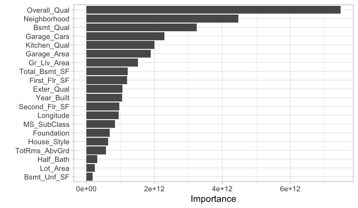

And similar the MARS model, since our relationship between our response variable and the predictor variables are non-linear, it becomes helpful to visualize the relationship between the most influential feature(s) and the response variable to see how they relate. Recall that we can do that with PDP plots.

Here, we see that the overall quality of a home doesn’t have a big impact unless the homes are rated very good to very excellent.

# prediction function
pdp_pred_fun <- function(object, newdata) {
  mean(predict(object, newdata, type = "numeric")$.pred)
}

# use the pdp package to extract partial dependence predictions
# and then plot
final_fit %>%
  pdp::partial(
   pred.var = "Overall_Qual", 
   pred.fun = pdp_pred_fun,
   grid.resolution = 10, 
   train = ames_train
  ) %>%
  ggplot(aes(Overall_Qual, yhat)) +
  geom_col() +
  scale_y_continuous(labels = scales::dollar)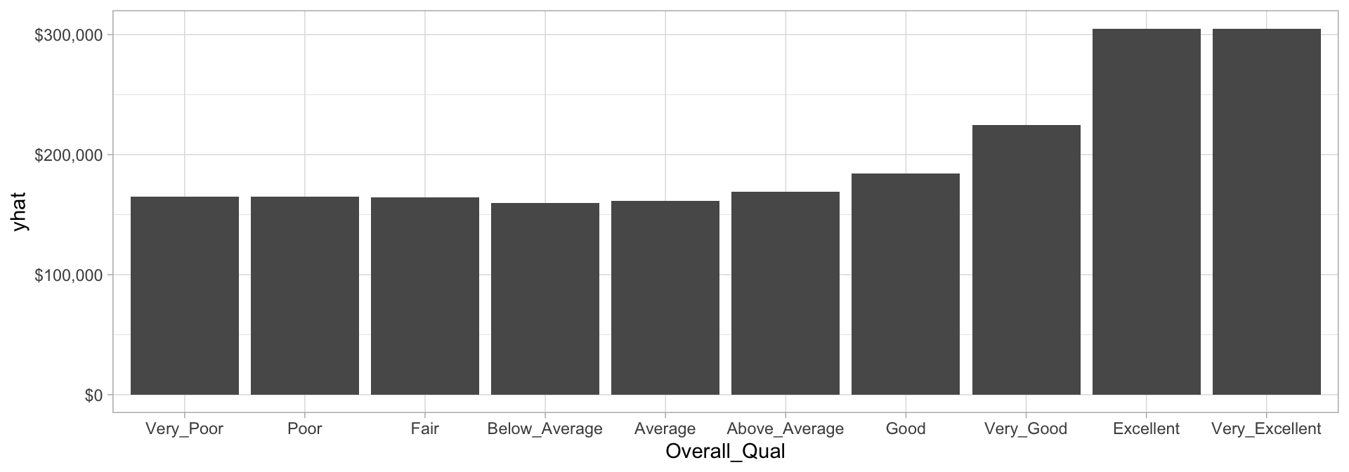

And if we do a similar plot for the Gr_Liv_Area variable we can see the non-linear relationship between the square footage of a home and the predicted Sale_Price that exists.

final_fit %>%
  pdp::partial(
   pred.var = "Gr_Liv_Area", 
   pred.fun = pdp_pred_fun,
   grid.resolution = 10, 
   train = ames_train
  ) %>%
   autoplot() +
   scale_y_continuous(labels = scales::dollar)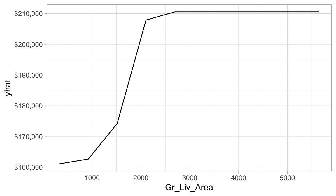

17.8.1 Knowledge check

Using the boston.csv dataset and the model from the previous Knowledge check that performed best…

• Plot the top 10 most influential features.
• Create and explain a PDP plot of the most influential feature.

17.9 Final thoughts

Decision trees have a number of advantages. Trees require very little pre-processing. This is not to say feature engineering may not improve upon a decision tree, but rather, that there are no pre-processing requirements. Monotonic transformations (e.g., \(\log\), \(\exp\), and \(\sqrt{}\)) are not required to meet algorithm assumptions as in many parametric models; instead, they only shift the location of the optimal split points. Outliers typically do not bias the results as much since the binary partitioning simply looks for a single location to make a split within the distribution of each feature.

Decision trees can easily handle categorical features without preprocessing. For unordered categorical features with more than two levels, the classes are ordered based on the outcome (for regression problems, the mean of the response is used and for classification problems, the proportion of the positive outcome class is used). For more details see J. Friedman, Hastie, and Tibshirani (2001), Breiman and Ihaka (1984), Ripley (2007), W. D. Fisher (1958), and Loh and Vanichsetakul (1988).

Missing values often cause problems with statistical models and analyses. Most procedures deal with them by refusing to deal with them—incomplete observations are tossed out. However, most decision tree implementations can easily handle missing values in the features and do not require imputation. This is handled in various ways but most commonly by creating a new “missing” class for categorical variables or using surrogate splits (see Therneau, Atkinson, et al. (1997) for details).

However, individual decision trees generally do not often achieve state-of-the-art predictive accuracy. In this module, we saw that the best pruned decision tree, although it performed better than linear regression, had a very poor RMSE (~$41,000) compared to some of the other models we’ve built. This is driven by the fact that decision trees are composed of simple yes-or-no rules that create rigid non-smooth decision boundaries. Furthermore, we saw that deep trees tend to have high variance (and low bias) and shallow trees tend to be overly bias (but low variance). In the modules that follow, we’ll see how we can combine multiple trees together into very powerful prediction models called ensembles.

17.10 Exercises

Using the same kernlab::spam data we saw in the section 12.10…

1. Split the data into 70-30 training-test sets.
2. Apply a decision tree classification model where type is our response variable and use all possible predictor variables.
   • Use a 5-fold cross-validation procedure.
   • Tune the cost complexity values with the default cost_complexity() values.
   • Tune the depth of the tree with the default tree_depth() values.
   • Tune the minimum number of observations in a node with the default min_n() values.
   • Assess a total of 5 values from each parameter (levels = 5).
3. Which model(s) have the highest AUC (roc_auc) scores?
4. What hyperparameter values provide these optimal results?
5. Use the hyperparameter values that provide the best results to finalize your workflow and and identify the top 20 most influential predictors.
6. Bonus: See if you can create a PDP plot for the #1 most influential variable. What does the relationship between this feature and the response variable look like?

References

Breiman, Leo. 1984. Classification and Regression Trees. Routledge.

Breiman, Leo, and Ross Ihaka. 1984. Nonlinear Discriminant Analysis via Scaling and ACE. Department of Statistics, University of California.

Fisher, Ronald A. 1936. “The Use of Multiple Measurements in Taxonomic Problems.” Annals of Eugenics 7 (2): 179–88.

Fisher, Walter D. 1958. “On Grouping for Maximum Homogeneity.” Journal of the American Statistical Association 53 (284): 789–98.

Friedman, Jerome, Trevor Hastie, and Robert Tibshirani. 2001. The Elements of Statistical Learning. Vol. 1. Springer Series in Statistics New York, NY, USA:

Hothorn, Torsten, Kurt Hornik, and Achim Zeileis. 2006. “Unbiased Recursive Partitioning: A Conditional Inference Framework.” Journal of Computational and Graphical Statistics 15 (3): 651–74.

Kass, Gordon V. 1980. “An Exploratory Technique for Investigating Large Quantities of Categorical Data.” Applied Statistics, 119–27.

Loh, Wei-Yin, and Nunta Vanichsetakul. 1988. “Tree-Structured Classification via Generalized Discriminant Analysis.” Journal of the American Statistical Association 83 (403): 715–25.

Quinlan, J Ross et al. 1996. “Bagging, Boosting, and C4. 5.” In AAAI/IAAI, Vol. 1, 725–30.

Quinlan, J. Ross. 1986. “Induction of Decision Trees.” Machine Learning 1 (1): 81–106.

Ripley, Brian D. 2007. Pattern Recognition and Neural Networks. Cambridge University Press.

Therneau, Terry M, Elizabeth J Atkinson, et al. 1997. “An Introduction to Recursive Partitioning Using the RPART Routines.” Mayo Foundation.

---

6. Other decision tree algorithms include the Iterative Dichotomiser 3 (J. Ross Quinlan 1986), C4.5 (J. Ross Quinlan et al. 1996), Chi-square automatic interaction detection (Kass 1980), Conditional inference trees (Hothorn, Hornik, and Zeileis 2006), and more.↩︎

7. Gini index and cross-entropy are the two most commonly applied loss functions used for decision trees. Classification error is rarely used to determine partitions as they are less sensitive to poor performing splits (J. Friedman, Hastie, and Tibshirani 2001).↩︎