18 Lesson 6b: Bagging

In an earlier module we learned about bootstrapping as a resampling procedure, which creates b new bootstrap samples by drawing samples with replacement of the original training data. This module illustrates how we can use bootstrapping to create an ensemble of predictions. Bootstrap aggregating, also called bagging, is one of the first ensemble algorithms⁸ machine learning practitioners learn and is designed to improve the stability and accuracy of regression and classification algorithms. By model averaging, bagging helps to reduce variance and minimize overfitting. Although it is usually applied to decision tree methods, it can be used with any type of method.

18.1 Learning objectives

By the end of this module you will know:

How and why bagging improves decision tree performance.
How to implement bagging and ensure you are optimizing bagging performance.
How to identify influential features and their effects on the response variable.

18.2 Prerequisites

# Helper packages
library(tidyverse)   # for data wrangling & plotting

# Modeling packages
library(tidymodels) 
library(baguette)    # you may need to install.packages this package

# Model interpretability packages
library(vip)         # for variable importance
library(pdp)         # for variable relationships

set.seed(123)
ames <- AmesHousing::make_ames()
split  <- initial_split(ames, prop = 0.7, strata = "Sale_Price")
ames_train  <- training(split)
ames_test   <- testing(split)

18.3 Why and when bagging works

Bootstrap aggregating (bagging) prediction models is a general method for fitting multiple versions of a prediction model and then combining (or ensembling) them into an aggregated prediction (Breiman 1996). Bagging is a fairly straight forward algorithm in which b bootstrap copies of the original training data are created, the regression or classification algorithm (commonly referred to as the base learner) is applied to each bootstrap sample and, in the regression context, new predictions are made by averaging the predictions together from the individual base learners. When dealing with a classification problem, the base learner predictions are combined using plurality vote or by averaging the estimated class probabilities together. This is represented in the below equation where $X$ is the record for which we want to generate a prediction, $\widehat{f_{bag}}$ is the bagged prediction, and $\widehat{f_1}\left(X\right), \widehat{f_2}\left(X\right), \dots, \widehat{f_b}\left(X\right)$ are the predictions from the individual base learners.

\[\begin{equation} \widehat{f_{bag}} = \widehat{f_1}\left(X\right) + \widehat{f_2}\left(X\right) + \cdots + \widehat{f_b}\left(X\right) \end{equation}\]

Because of the aggregation process, bagging effectively reduces the variance of an individual base learner (i.e., averaging reduces variance); however, bagging does not always improve upon an individual base learner. As discussed in our bias vs variance discussion, some models have larger variance than others. Bagging works especially well for unstable, high variance base learners—algorithms whose predicted output undergoes major changes in response to small changes in the training data (Dietterich 2000b, 2000a). This includes algorithms such as decision trees and KNN (when k is sufficiently small). However, for algorithms that are more stable or have high bias, bagging offers less improvement on predicted outputs since there is less variability (e.g., bagging a linear regression model will effectively just return the original predictions for large enough $b$).

The general idea behind bagging is referred to as the “wisdom of the crowd” effect and was popularized by Surowiecki (2005). It essentially means that the aggregation of information in large diverse groups results in decisions that are often better than could have been made by any single member of the group. The more diverse the group members are then the more diverse their perspectives and predictions will be, which often leads to better aggregated information. Think of estimating the number of jelly beans in a jar at a carinival. While any individual guess is likely to be way off, you’ll often find that the averaged guesses tends to be a lot closer to the true number.

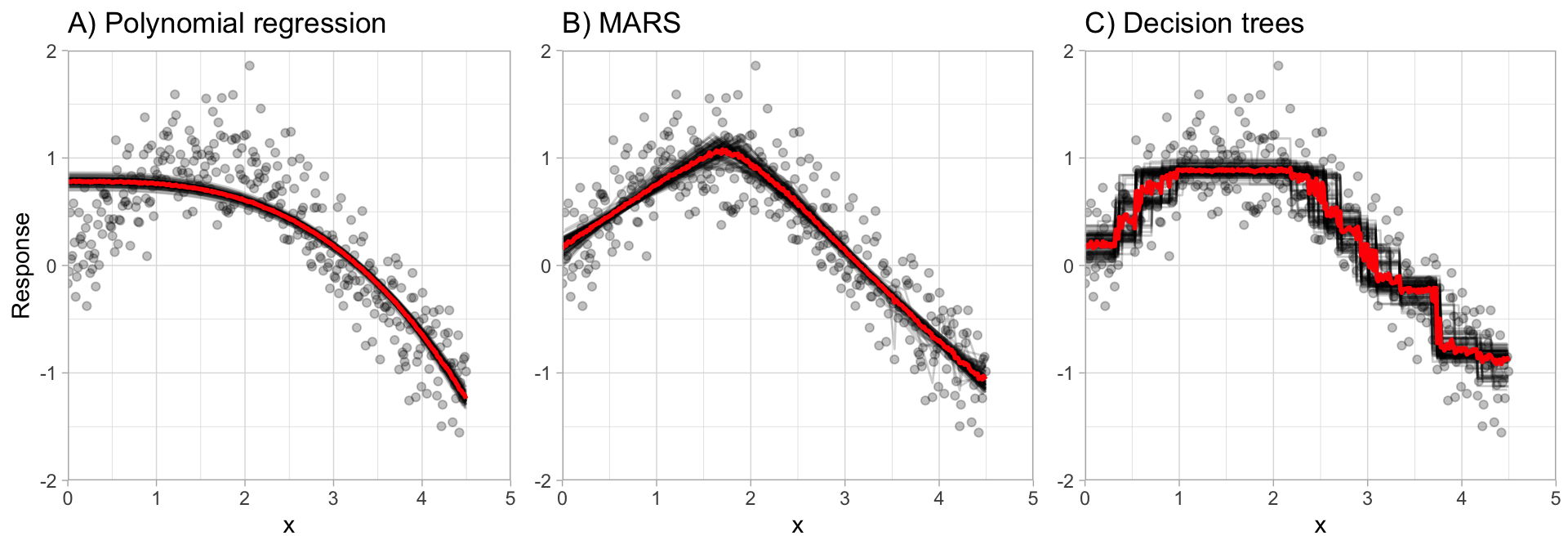
This is illustrated in the below plot, which compares bagging $b = 100$ polynomial regression models, MARS models, and CART decision trees. You can see that the low variance base learner (polynomial regression) gains very little from bagging while the higher variance learner (decision trees) gains significantly more. Not only does bagging help minimize the high variability (instability) of single trees, but it also helps to smooth out the prediction surface.

Optimal performance is often found by bagging 50–500 trees. Data sets that have a few strong predictors typically require less trees; whereas data sets with lots of noise or multiple strong predictors may need more. Using too many trees will not lead to overfitting. However, it’s important to realize that since multiple models are being run, the more iterations you perform the more computational and time requirements you will have. As these demands increase, performing k-fold CV can become computationally burdensome.

A benefit to creating ensembles via bagging, which is based on resampling with replacement, is that it can provide its own internal estimate of predictive performance with the out-of-bag (OOB) sample. The OOB sample can be used to test predictive performance and the results usually compare well compared to k-fold CV assuming your data set is sufficiently large (say $n \geq 1,000$). Consequently, as your data sets become larger and your bagging iterations increase, it is common to use the OOB error estimate as a proxy for predictive performance.

Think of the OOB estimate of generalization performance as an unstructured, but free CV statistic.

18.4 Fitting a bagged decision tree model

Recall in the decision tree module that our optimally tuned single decision tree model was obtaining a mid-$30K RMSE. In this first implementation we’ll perform the same process; however, instead of a single decision tree we’ll use bagging to create and aggregate performance across 5 bagged trees.

In R we use baguette::bag_tree to create a bagged tree model object, which can be applied to decision tree or MARS models. Note how we do not need to perform any feature engineering as decision trees (and therefore bagged decision trees) can handle numeric and categorical features just as they are.

Note how aggregating just 5 decision trees improves our RMSE to around $30K.

# create model recipe with all features
model_recipe <- recipe(
    Sale_Price ~ ., 
    data = ames_train
  )

# create bagged CART model object and
# start with 5 bagged trees
tree_mod <- bag_tree() %>%
  set_engine("rpart", times = 5) %>%
  set_mode("regression")

# create resampling procedure
set.seed(13)
kfold <- vfold_cv(ames_train, v = 5)

# train model
results <- fit_resamples(tree_mod, model_recipe, kfold)

# model results
collect_metrics(results)
## # A tibble: 2 × 6
##   .metric .estimator      mean     n std_err
##   <chr>   <chr>          <dbl> <int>   <dbl>
## 1 rmse    standard   29850.        5 1.27e+3
## 2 rsq     standard       0.861     5 1.45e-2
## # ℹ 1 more variable: .config <chr>

18.4.1 Knowledge check

Using the boston.csv dataset:

Apply a bagged decision tree model where cmedv is the response variable and use all possible predictor variables. Use a 5-fold cross validation procedure to assess…

Bagging 5 trees
Bagging 10 trees
Bagging 25 trees

How does the model perform in each scenario? Do adding more trees improve performance?

18.5 Tuning

One thing to note is that typically, the more trees the better. As we add more trees we’re averaging over more high variance decision trees. Early on, we see a dramatic reduction in variance (and hence our error) but eventually the error will typically flatline and stabilize signaling that a suitable number of trees has been reached. Often, we need only 50–100 trees to stabilize the error (in other cases we may need 500 or more).

Consequently, we can treat the number of trees as a tuning parameter where our focus is to make sure we are using enough trees for our error metric to converge at a optimal value (minimize RMSE in our case). However, rarely do we run the risk of including too many trees as we typically will not see our error metric degrade after adding more trees than necessary.

The primary concern is compute efficiency, we want enough trees to reach an optimal resampling error; however, not more trees than necessary as it will slow down computational efficiency.

In this example we use a hyperparameter grid to assess 5, 25, 50, 100, and 200 trees. We see an initial decrease but as we start using 50+ trees we only see marginal changes in our RMSE, suggesting we have likely reached enough trees to minimize the RMSE and any additional differences are likely due to the standard error that occurs during the bootstrapping process.

# create bagged CART model object with
# tuning option set for number of bagged trees
tree_mod <- bag_tree() %>%
  set_engine("rpart", times = tune()) %>%
  set_mode("regression")

# create the hyperparameter grid
hyper_grid <- expand.grid(times = c(5, 25, 50, 100, 200))

# train our model across the hyperparameter grid
set.seed(123)
results <- tune_grid(tree_mod, model_recipe, resamples = kfold, grid = hyper_grid)


# model results
show_best(results, metric = "rmse")
## # A tibble: 5 × 7
##   times .metric .estimator   mean     n
##   <dbl> <chr>   <chr>       <dbl> <int>
## 1   200 rmse    standard   26175.     5
## 2   100 rmse    standard   26430.     5
## 3    50 rmse    standard   26536.     5
## 4    25 rmse    standard   26909.     5
## 5     5 rmse    standard   30276.     5
## # ℹ 2 more variables: std_err <dbl>,
## #   .config <chr>

When bagging trees we can also tune the same hyperparameters that we tuned with decision trees (cost_complexity, tree_depth, min_n). See bag_tree? for details.

However, the default values for these hyperparameters is set to grow our trees to the maximum depth and not prune them at all. It has been shown that bagging many deep, overfit trees typically leads to best performance.

18.5.1 Knowledge check

Using the boston.csv dataset:

Apply a bagged decision tree model where cmedv is the response variable and use all possible predictor variables. Use a 5-fold cross validation procedure and tune the number of trees to assess 5, 10, 25, 50, 100, and 150 trees.

How does the model perform in each scenario? Do adding more trees improve performance? At what point do we experience diminishing returns in our cross-validated RMSE?

18.6 Feature interpretation

Unfortunately, due to the bagging process, models that are normally perceived as interpretable are no longer so. However, we can still make inferences about how features are influencing our model. Recall in the decision tree module that we measure feature importance based on the sum of the reduction in the loss function (e.g., SSE) attributed to each variable at each split in a given tree.

For bagged decision trees, this process is similar. For each tree, we compute the sum of the reduction of the loss function across all splits. We then aggregate this measure across all trees for each feature. The features with the largest average decrease in SSE (for regression) are considered most important.

The following extracts the feature importance for our best performing bagged decision trees. Unfortunately, vip::vip() doesn’t work naturally with models from bag_tree so we need to manually extract the variable importance scores and plot them with ggplot. We see that Overall_Qual and Neighborhood are the top two most influential features.

# identify best model
best_hyperparameters <- results %>%
   select_best("rmse")

# finalize workflow object
final_wf <- workflow() %>%
   add_recipe(model_recipe) %>%
   add_model(tree_mod) %>%
   finalize_workflow(best_hyperparameters)

# final fit on training data
final_fit <- final_wf %>%
   fit(data = ames_train)

# plot top 20 influential variables
vi <- final_fit %>%
   extract_fit_parsnip() %>%
   .[['fit']] %>%
   var_imp() %>%
   slice(1:20)

ggplot(vi, aes(value, reorder(term, value))) +
   geom_col() +
   ylab(NULL) +
   xlab("Feature importance")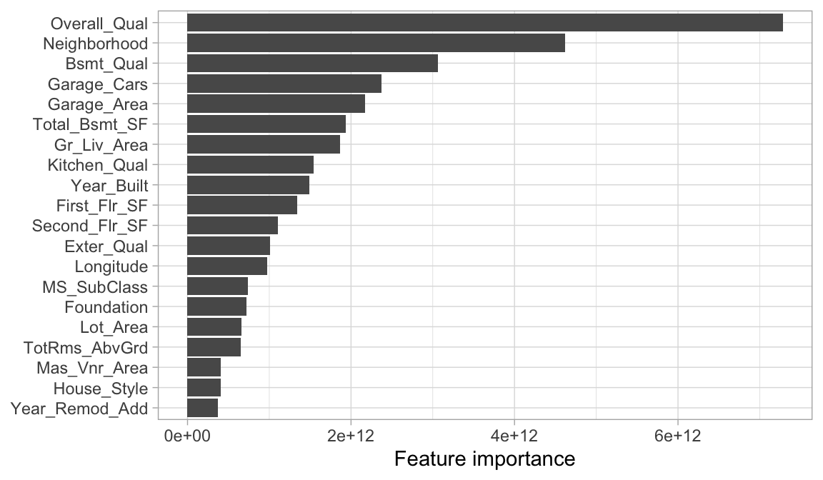

We can then plot the partial dependence of the most influential feature to see how it influences the predicted values. We see that as overall quality increase we see a significant increase in the predicted sale price.

# prediction function
pdp_pred_fun <- function(object, newdata) {
   predict(object, newdata, type = "numeric")$.pred
}

# use the pdp package to extract partial dependence predictions
# and then plot
final_fit %>%
   pdp::partial(
     pred.var = "Overall_Qual", 
     pred.fun = pdp_pred_fun,
     grid.resolution = 10, 
     train = ames_train
   ) %>%
  ggplot(aes(Overall_Qual, yhat)) +
    geom_boxplot() +
    scale_y_continuous(labels = scales::dollar)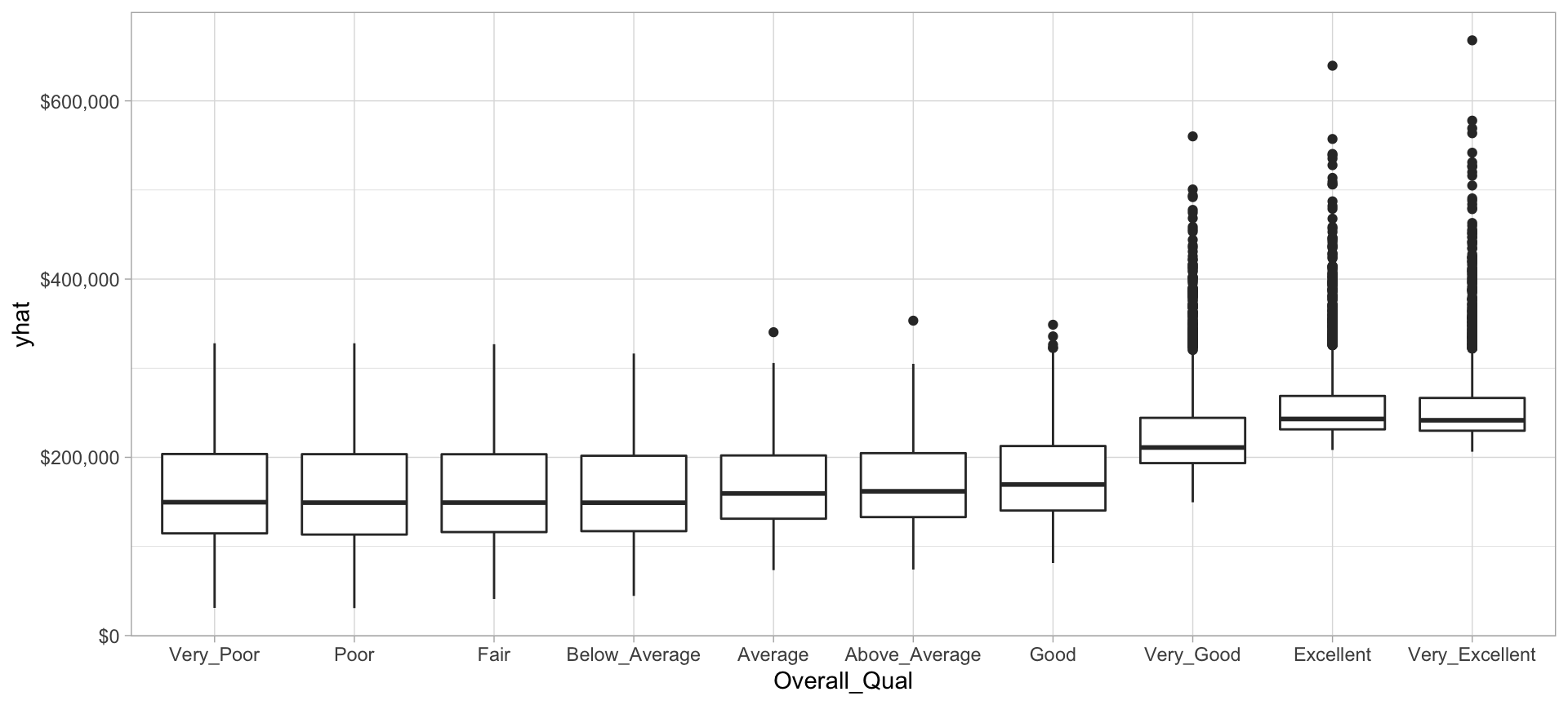

Now let’s plot the PDP for the Gr_Liv_Area and see how that variable relates to the predicted sale price.

# prediction function
pdp_pred_fun <- function(object, newdata) {
   mean(predict(object, newdata, type = "numeric")$.pred)
}

# use the pdp package to extract partial dependence predictions
# and then plot
final_fit %>%
   pdp::partial(
     pred.var = "Gr_Liv_Area", 
     pred.fun = pdp_pred_fun,
     grid.resolution = 10, 
     train = ames_train
   ) %>%
   autoplot() +
   scale_y_continuous(labels = scales::dollar)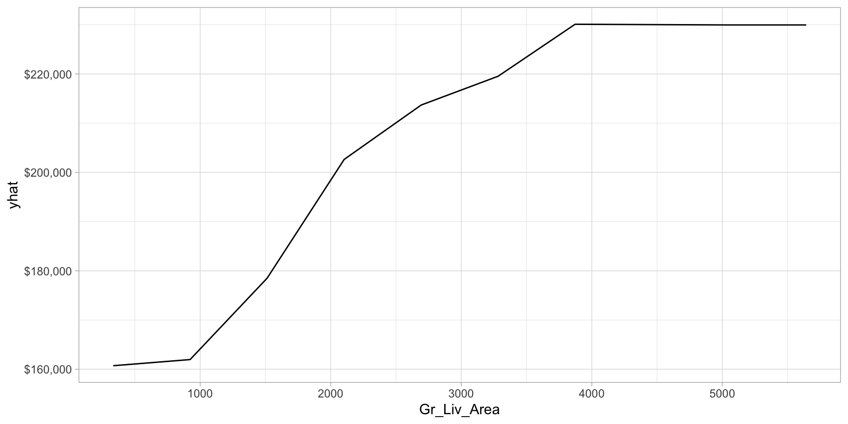

18.6.1 Knowledge check

Using the boston.csv dataset and the model from the previous Knowledge check that performed best…

Plot the top 10 most influential features.
Create and explain a PDP plot of the most influential feature.

18.7 Final thoughts

Bagging improves the prediction accuracy for high variance (and low bias) models at the expense of interpretability and computational speed. However, using various interpretability algorithms such as VIPs and PDPs, we can still make inferences about how our bagged model leverages feature information. Also, since bagging consists of independent processes, the algorithm is easily parallelizable.

However, when bagging trees, a problem still exists. Although the model building steps are independent, the trees in bagging are not completely independent of each other since all the original features are considered at every split of every tree. Rather, trees from different bootstrap samples typically have similar structure to each other (especially at the top of the tree) due to any underlying strong relationships.

For example, if we create six decision trees with different bootstrapped samples of the Boston housing data (Harrison Jr and Rubinfeld 1978), we see a similar structure as the top of the trees. Although there are 15 predictor variables to split on, all six trees have both lstat and rm variables driving the first few splits.

We use the Boston housing data in this example because it has fewer features and shorter names than the Ames housing data. Consequently, it is easier to compare multiple trees side-by-side; however, the same tree correlation problem exists in the Ames bagged model.

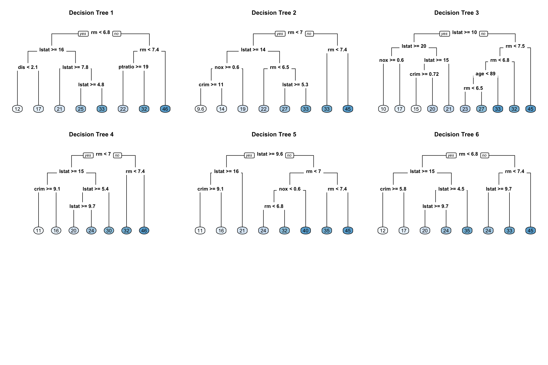
Figure 18.1: Six decision trees based on different bootstrap samples.

In the next lesson we’ll see how to resolve this concern using a modification of bagged trees called random forest.

18.8 Exercises

Using the same kernlab::spam data we saw in the section 12.10…

Split the data into 70-30 training-test sets.
Apply a bagged decision tree model modeling the type response variable as a function of all available features.
How many trees are required before the loss function stabilizes?
How does the model performance compare to the decision tree model applied in the previous lesson’s exercise?
Which 10 features are considered most influential? Are these the same features that have been influential in previous model?
Create partial dependence plots for the top two most influential features. Explain the relationship between the feature and the predicted values.

References

———. 1996. “Bagging Predictors.” Machine Learning 24 (2): 123–40.

Dietterich, Thomas G. 2000a. “An Experimental Comparison of Three Methods for Constructing Ensembles of Decision Trees: Bagging, Boosting, and Randomization.” Machine Learning 40 (2): 139–57.

———. 2000b. “Ensemble Methods in Machine Learning.” In International Workshop on Multiple Classifier Systems, 1–15. Springer.

Harrison Jr, David, and Daniel L Rubinfeld. 1978. “Hedonic Housing Prices and the Demand for Clean Air.” Journal of Environmental Economics and Management 5 (1): 81–102.

Surowiecki, James. 2005. The Wisdom of Crowds. Anchor.

Also commonly referred to as a meta-algorithm.↩︎