11 Lesson 4a: Logistic Regression
Linear regression is used to approximate the (linear) relationship between a continuous response variable and a set of predictor variables. However, when the response variable is binary (i.e., Yes/No), linear regression is not appropriate. Fortunately, analysts can turn to an analogous method, logistic regression, which is similar to linear regression in many ways. This module explores the use of logistic regression for binary response variables. Logistic regression can be expanded for problems where the response variable has more than two categories (i.e. High/Medium/Low, Flu/Covid/Allergies, Win/Lose/Tie); however, that goes beyond our intent here (see Faraway (2016a) for discussion of multinomial logistic regression in R).
11.1 Learning objectives
By the end of this module you will:
- Understand why linear regression does not work for binary response variables.
- Know how to apply and interpret simple and multiple logistic regression models.
- Know how to assess model accuracy of various logistic regression models.
11.2 Prerequisites
For this section we’ll use the following packages:
# Helper packages
library(tidyverse) # for data wrangling & plotting

# Modeling packages
library(tidymodels)

# Model interpretability packages
library(vip)      # variable importance
To illustrate logistic regression concepts we’ll use the employee attrition data, where our intent is to predict the Attrition response variable (coded as "Yes"/"No"). As in the previous module, we’ll set aside 30% of our data as a test set to assess our generalizability error.
churn_data_path <- here::here("data", "attrition.csv")
churn <- read_csv(churn_data_path)

# Recode response variable as a factor
churn <- mutate(churn, Attrition = factor(Attrition))

# Create training (70%) and test (30%) sets
set.seed(123)  # for reproducibility
churn_split <- initial_split(churn, prop = .7, strata = "Attrition")
churn_train <- training(churn_split)
churn_test  <- testing(churn_split)
11.3 Why logistic regression
To provide a clear motivation for logistic regression, assume we have credit card default data for customers and we want to understand if the current credit card balance of a customer is an indicator of whether or not they’ll default on their credit card. To classify a customer as a high- vs. low-risk defaulter based on their balance we could use linear regression; however, the left plot below illustrates how linear regression would predict the probability of defaulting. Unfortunately, for balances close to zero we predict a negative probability of defaulting; if we were to predict for very large balances, we would get values bigger than 1. These predictions are not sensible, since of course the true probability of defaulting, regardless of credit card balance, must fall between 0 and 1. These inconsistencies only increase as our data become more imbalanced and the number of outliers increase. Contrast this with the logistic regression line (right plot) that is nonlinear (sigmoidal-shaped).
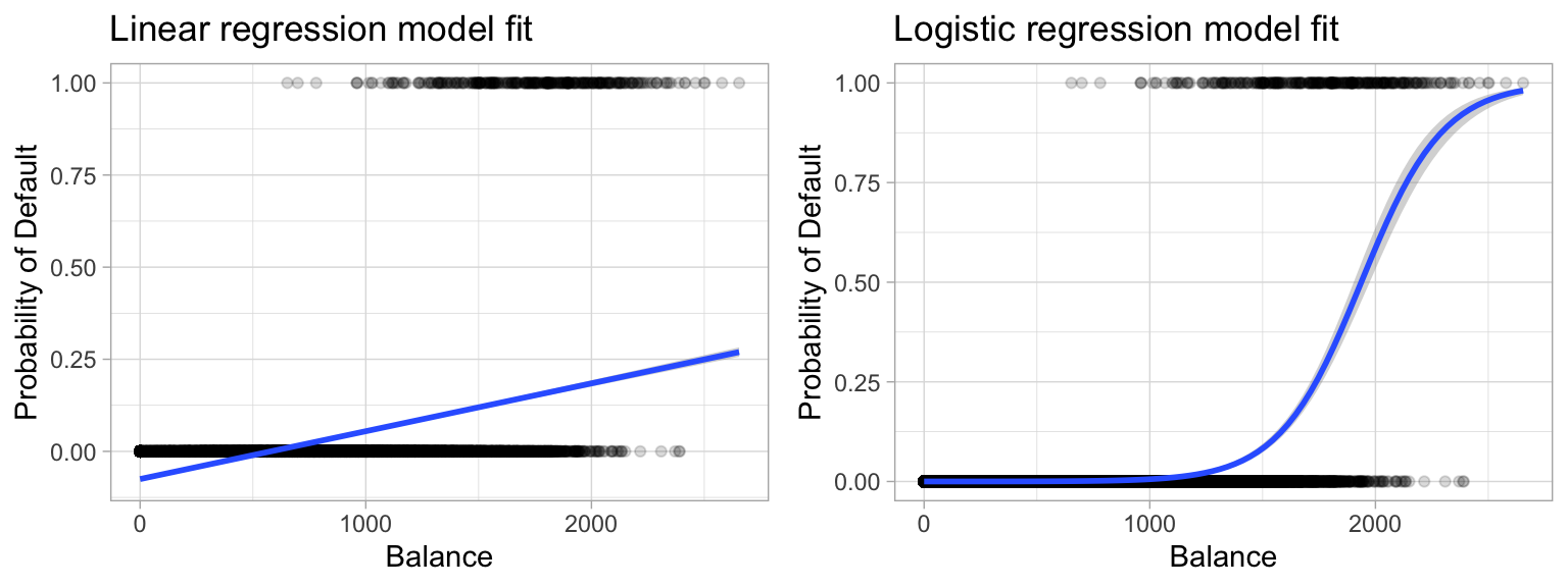
Figure 11.1: Comparing the predicted probabilities of linear regression (left) to logistic regression (right). Predicted probabilities using linear regression results in flawed logic whereas predicted values from logistic regression will always lie between 0 and 1.
To avoid the inadequacies of the linear model fit on a binary response, we must model the probability of our response using a function that gives outputs between 0 and 1 for all values of \(x\). Many functions meet this description. In logistic regression, we use the logistic function, which is defined as the following equation and produces the S-shaped curve in the right plot above.
\[\begin{equation} p\left(x\right) = \frac{e^{b_0 + b_1x}}{1 + e^{b_0 + b_1x}} \end{equation}\]
The \(b_i\) parameters represent the coefficients as in linear regression and \(p\left(x\right)\) may be interpreted as the probability that the positive class (default in the above example) is present. The minimum for \(p\left(x\right)\) is obtained at \(\lim_{a \rightarrow -\infty} \left[ \frac{e^a}{1+e^a} \right] = 0\), and the maximum for \(p\left(x\right)\) is obtained at \(\lim_{a \rightarrow \infty} \left[ \frac{e^a}{1+e^a} \right] = 1\) which restricts the output probabilities to 0–1. Rearranging the above equation yields the logit transformation (which is where logistic regression gets its name):
\[\begin{equation} g\left(x\right) = \ln \left[ \frac{p\left(x\right)}{1 - p\left(x\right)} \right] = b_0 + b_1 x \end{equation}\]
Applying a logit transformation to \(p\left(x\right)\) results in a linear equation similar to the mean response in a simple linear regression model. Using the logit transformation also results in an intuitive interpretation for the magnitude of \(b_1\): the odds (e.g., of defaulting) increase multiplicatively by \(\exp\left(b_1\right)\) for every one-unit increase in \(x\). A similar interpretation exists if \(x\) is categorical; see Agresti (2003), Chapter 5, for more details.
This may seem overwhelming but don’t worry, the meaning of this math and how you interpret the predictor variable coefficients will become clearer later in this lesson. Your main take-away is that logistic regression:
- Models the probability of our response using a function that restricts this probability to be between 0 and 1.
- The coefficients of our logistic regression represent the multiplicative increase in the odds of our response variable for every one-unit increase in \(x\).
11.4 Simple logistic regression
We will fit two logistic regression models in order to predict the probability of an employee attriting. The first predicts the probability of attrition based on their monthly income (MonthlyIncome) and the second is based on whether or not the employee works overtime (OverTime).
To simplify the code we do not run cross validation procedures. We will in a later section but for now we simply want to get a grasp of interpreting a logistic regression model.
We use logistic_reg() for our model object. Note that we do not set the engine for this model type. This means we will use the default engine, which is the glm package (see ?logistic_reg for details).
11.5 Interpretation
Bear in mind that the coefficient estimates from logistic regression characterize the relationship between the predictor and response variable on a log-odds (i.e., logit) scale. Unlike, linear regression, this can make interpretation of coefficients difficult. At a macro level, larger coefficients suggest that that feature increases the odds of the response more than smaller valued coefficients.
However, for our purpose, it is easier to focus on the interpretation of the output. The following predicts the probability of employee attrition based on the two models we fit. So in this example, for the first observation our model predicts there is a 78% probability that the employee will not leave and a 22% probability that they will.
lr_fit1 %>% predict(churn_train, type = "prob")
## # A tibble: 1,028 × 2
##    .pred_No .pred_Yes
##       <dbl>     <dbl>
##  1    0.784    0.216
##  2    0.778    0.222
##  3    0.779    0.221
##  4    0.834    0.166
##  5    0.772    0.228
##  6    0.813    0.187
##  7    0.784    0.216
##  8    0.906    0.0937
##  9    0.954    0.0463
## 10    0.807    0.193
## # ℹ 1,018 more rows
Let’s use these predictions to assess how our logistic regression model views the relationship between our predictor variables and the response variable. In the first plot, we can see that as MonthlyIncome increases, the predicted probability of attrition decreases from a little over 0.25 to 0.025.
If we look at the second plot, which plots the predicted probability of Attrition based on whether employees work OverTime. We can see that employees that work overtime have a 0.3 probability of attrition while those that don’t work overtime only have a 0.1 probability of attrition. Basically, working overtimes increases the probability of employee churn by a factor of 3!
p1 <- lr_fit1 %>%
 predict(churn_train, type = "prob") %>%
 mutate(MonthlyIncome = churn_train$MonthlyIncome) %>%
 ggplot(aes(MonthlyIncome, .pred_Yes)) +
 geom_point(alpha = .2) +
 scale_y_continuous("Probability of Attrition", limits = c(0, 1)) +
 ggtitle("Predicted probabilities for lr_fit1")

p2 <- lr_fit2 %>%
 predict(churn_train, type = "prob") %>%
 mutate(OverTime = churn_train$OverTime) %>%
 ggplot(aes(OverTime, .pred_Yes, color = OverTime)) +
 geom_boxplot(show.legend = FALSE) +
 geom_rug(sides = "b", position = "jitter", alpha = 0.2, show.legend = FALSE) +
  scale_y_continuous("Probability of Attrition", limits = c(0, 1)) +
  ggtitle("Predicted probabilities for lr_fit2")

gridExtra::grid.arrange(p1, p2, nrow = 1)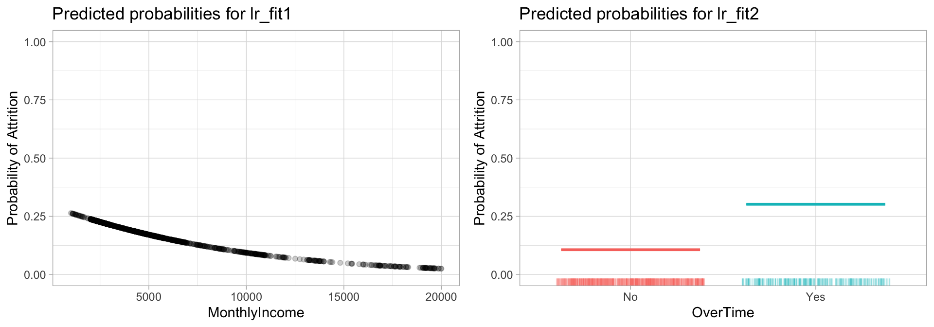
Figure 11.2: Predicted probablilities of employee attrition based on monthly income (left) and overtime (right). As monthly income increases, lr_fit1 predicts a decreased probability of attrition and if employees work overtime lr_fit2 predicts an increased probability.
The table below shows the coefficient estimates and related information that result from fitting a logistic regression model in order to predict the probability of Attrition = Yes for our two models. Bear in mind that the coefficient estimates from logistic regression characterize the relationship between the predictor and response variable on a log-odds (i.e., logit) scale.
For lr_fit1, the estimated coefficient for MonthlyIncome is -0.000139, which is negative, indicating that an increase in MonthlyIncome is associated with a decrease in the probability of attrition. Similarly, for lr_fit2, employees who work OverTime are associated with an increased probability of attrition compared to those that do not work OverTime.
tidy(lr_fit1)
## # A tibble: 2 × 5
##   term           estimate std.error statistic      p.value
##   <chr>             <dbl>     <dbl>     <dbl>        <dbl>
## 1 (Intercept)   -0.886    0.157         -5.64 0.0000000174
## 2 MonthlyIncome -0.000139 0.0000272     -5.10 0.000000344

tidy(lr_fit2)
## # A tibble: 2 × 5
##   term        estimate std.error statistic  p.value
##   <chr>          <dbl>     <dbl>     <dbl>    <dbl>
## 1 (Intercept)    -2.13     0.119    -17.9  1.46e-71
## 2 OverTimeYes     1.29     0.176      7.35 2.01e-13
As discussed earlier, it is easier to interpret the coefficients using an exp() transformation:
exp(coef(lr_fit1$fit))
##   (Intercept) MonthlyIncome
##     0.4122647     0.9998614
exp(coef(lr_fit2$fit))
## (Intercept) OverTimeYes
##   0.1189759   3.6323389
Thus, the odds of an employee attriting in lr_fit1 increase multiplicatively by 0.9999 for every one dollar increase in MonthlyIncome, whereas the odds of attriting in lr_fit2 increase multiplicatively by 3.632 for employees that work OverTime compared to those that do not.
Many aspects of the logistic regression output are similar to those discussed for linear regression. For example, we can use the estimated standard errors to get confidence intervals as we did for linear regression.
confint(lr_fit1$fit) # for odds, you can use `exp(confint(model1))`
##                       2.5 %        97.5 %
## (Intercept)   -1.1932606571 -5.761048e-01
## MonthlyIncome -0.0001948723 -8.803311e-05
confint(lr_fit2$fit)
##                  2.5 %    97.5 %
## (Intercept) -2.3695727 -1.902409
## OverTimeYes  0.9463761  1.635373
11.5.1 Knowledge check
-
Load the spam data set from the kernlab package with the code below.
Review the data documentation with
?spam. - What is the response variable?
- Split the data into a train and test set using a 70-30 split.
-
Pick a single predictor variable and apply a simple logistic
regression model that models the
typevariable as a function of that predictor variable. - Interpret the feature’s coefficient
11.6 Multiple logistic regression
We can also extend our model as seen in our earlier equation so that we can predict a binary response using multiple predictors:
\[\begin{equation} p\left(X\right) = \frac{e^{b_0 + b_1 x_1 + \cdots + b_p x_p }}{1 + e^{b_0 + b_1 x_1 + \cdots + b_p x_p}} \end{equation}\]
Let’s go ahead and fit a model that predicts the probability of Attrition based on the MonthlyIncome and OverTime. Our results show that both features have an impact on employee attrition; however, working OverTime tends to nearly double the probability of attrition!
# model 3
lr_fit3 <- lr_mod %>%
  fit(Attrition ~ MonthlyIncome + OverTime, data = churn_train)

tidy(lr_fit3)
## # A tibble: 3 × 5
##   term           estimate std.error statistic  p.value
##   <chr>             <dbl>     <dbl>     <dbl>    <dbl>
## 1 (Intercept)   -1.33     0.177         -7.54 4.74e-14
## 2 MonthlyIncome -0.000147 0.0000280     -5.27 1.38e- 7
## 3 OverTimeYes    1.35     0.180          7.50 6.59e-14
lr_fit3 %>%
predict(churn_train, type = "prob") %>%
mutate(
MonthlyIncome = churn_train$MonthlyIncome,
OverTime = churn_train$OverTime
) %>%
ggplot(aes(MonthlyIncome, .pred_Yes, color = OverTime)) +
geom_point(alpha = 0.5, size = 0.8) +
scale_y_continuous("Probability of Attrition", limits = c(0, 1)) +
ggtitle("Predicted probabilities for lr_fit3")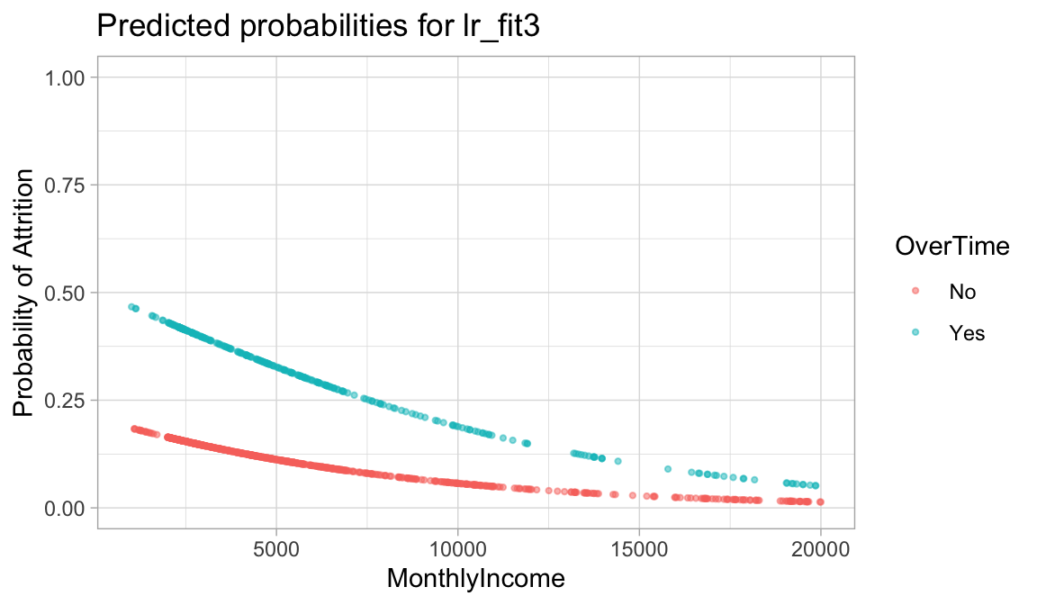
11.7 Assessing model accuracy
With a basic understanding of logistic regression under our belt, similar to linear regression our concern now shifts to how well our models predict. As discussed in lesson 1b, there are multiple metrics we can use for classification models.
11.7.1 Accuracy
The most basic classification metric is accuracy rate. This answers the question - “Overall, how often is the classifier correct?” Our objective is to maximize this metric. We can compute the accuracy with accuracy().
Here, we compute our error metric with the test data but we’ll show shortly how to do so using resampling procedures as we learned about in the last lesson.
# accuracy of our first model
lr_fit1 %>%
   predict(churn_test) %>%
   bind_cols(churn_test %>% select(Attrition)) %>%
   accuracy(truth = Attrition, estimate = .pred_class)
## # A tibble: 1 × 3
##   .metric  .estimator .estimate
##   <chr>    <chr>          <dbl>
## 1 accuracy binary         0.837
Unfortunately, the accuracy rate only tells us how many predictions were correct versus not. Sometimes we may want to understand more behind how our predictions are correct vs incorrect. To do so we can use…
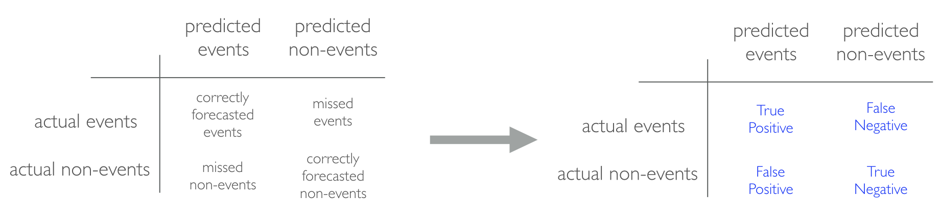
11.7.2 Confusion matrix
When applying classification models, we often use a confusion matrix to evaluate certain performance measures. A confusion matrix is simply a matrix that compares actual categorical levels (or events) to the predicted categorical levels. When we predict the right level, we refer to this as a true positive. However, if we predict a level or event that did not happen this is called a false positive (i.e. we predicted an employee would leave and they did not). Alternatively, when we do not predict a level or event and it does happen that this is called a false negative (i.e. an employee that we did not predict to leave does).
We can get the confusion matrix for a given fit model with conf_mat(). These results provide us with some very useful information. For lr_fit1, our model is predicting “No” for every observation!
lr_fit1 %>%
   predict(churn_test) %>%
   bind_cols(churn_test %>% select(Attrition)) %>%
   conf_mat(truth = Attrition, estimate = .pred_class)
##           Truth
## Prediction  No Yes
##        No  370  72
##        Yes   0   0
For a better example, let’s train a model with all predictor variables. Now when we create our confusion matrix we see that our model predicts yes’s and no’s.
lr_fit4 <- lr_mod %>%
  fit(Attrition ~ ., data = churn_train)

lr_fit4 %>%
   predict(churn_test) %>%
   bind_cols(churn_test %>% select(Attrition)) %>%
   conf_mat(truth = Attrition, estimate = .pred_class)
##           Truth
## Prediction  No Yes
##        No  353  38
##        Yes  17  34
Using a confusion matrix can allow us to extract different meaningful metrics for our binary classifier. For example, given the above confusion matrix we can assess the following:
- Our model does far better at accurately predicting when an employee is not going to leave (Prediction = No & Truth = No) versus accurately predicting when an employee is going to leave (Prediction = Yes & Truth = Yes).
- When our model is inaccurate, we can see that it is from more false negatives (Prediction = No but Truth = Yes) than false positives (Prediction = Yes but Truth = No). This means our model is biased towards predicting that an employee is going to stay when in fact they end up leaving.
When assessing model performance for a classification model, understanding how our model errors with false negatives and false positives is important. This information can be helpful to decision makers.
Often, we want a classifier that has high accuracy and does well when it predicts an event will and will not occur, which minimizes false positives and false negatives. One way to capture this is with area under the curve.
11.7.3 Area under the curve
Area under the curve (AUC) is an approach that plots the false positive rate along the x-axis and the true positive rate along the y-axis. Technically, we call this plot the Receiver Operator Curve (ROC). A line that is diagonal from the lower left corner to the upper right corner represents a random guess. The higher the line is in the upper left-hand corner, the better. The AUC metric computes the area under the ROC; so our objective is to maximize the AUC value.
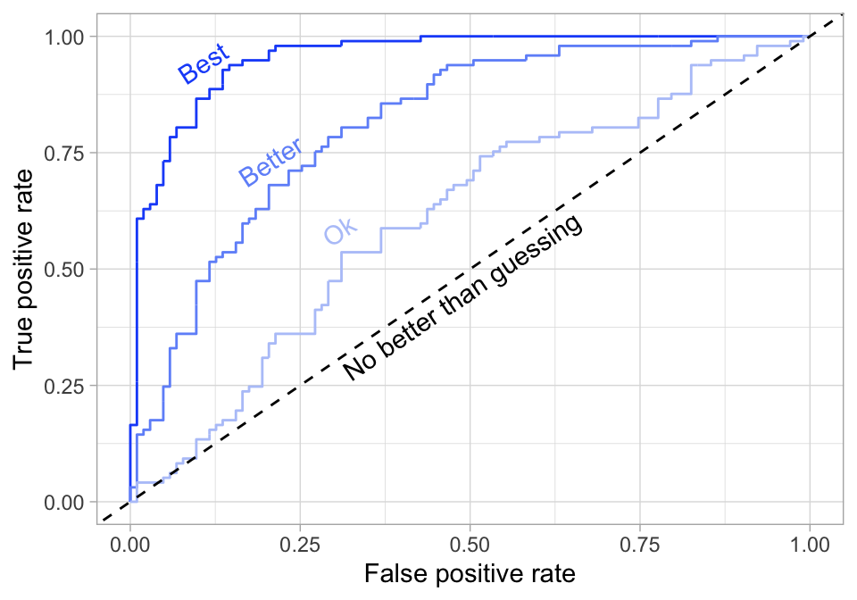
Figure 11.3: ROC curve.
For our logistic regression model we can get the ROC curve with the following:
Notice how the y-axis is called “sensitivity” and the x-axis is “1=specificity”. These are just alternative terms referring to “true positive rate” and “false positive rate” respectively.
lr_fit4 %>%
   predict(churn_train, type = "prob") %>%
   mutate(truth = churn_train$Attrition) %>%
   roc_curve(truth, .pred_No) %>%
   autoplot()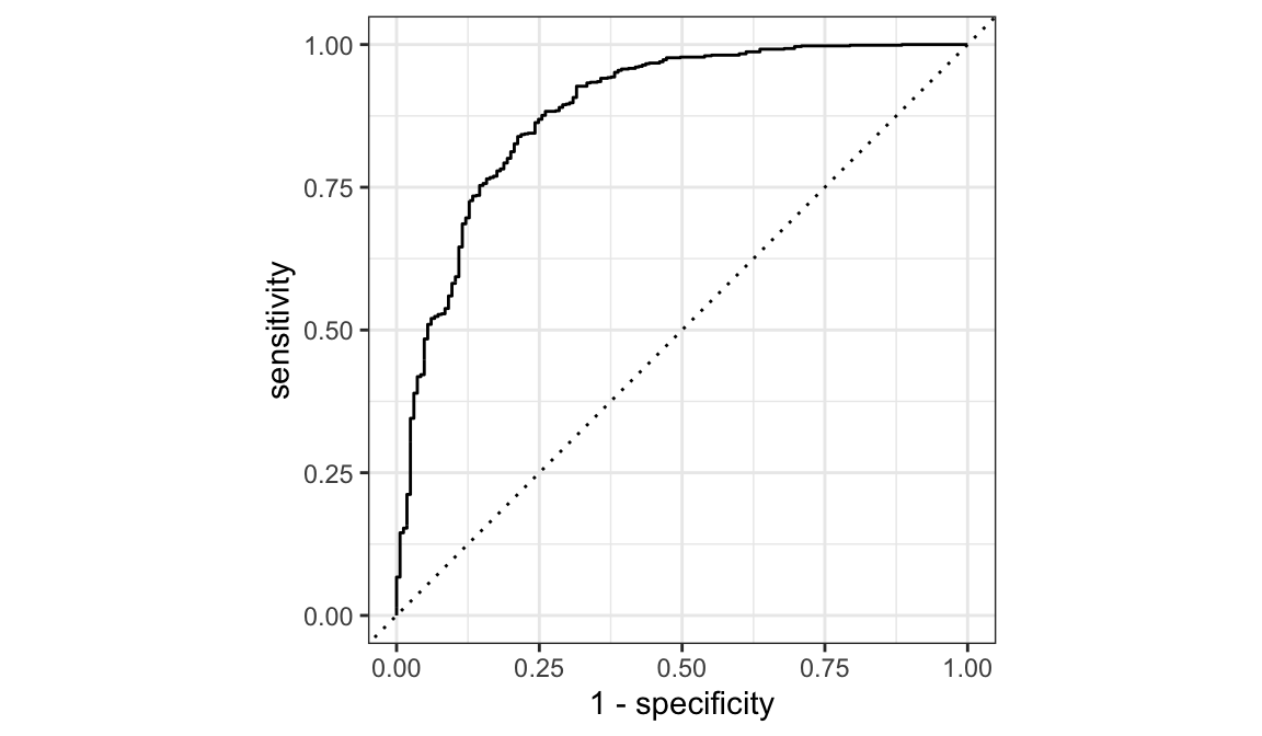
And we can compute the AUC metric with roc_auc():
11.7.4 Knowledge check
Using the same spam data as in the previous Knowledge check…
-
Apply a logistic regression model that models the
typevariable as a function of all predictor variables. - Assess the accuracy of this model on the test data.
- Assess and interpret the confusion matrix results for this model on the test data.
- Plot the ROC curve for this model and compute the AUC (using the test data).
11.8 Cross-validation performance
However, recall that our previous models were not based on cross validation procedures. If we re-perform our analysis using a 5-fold cross validation procedure we see that our average AUC metric is lower than the test set. This is probably a better indicator on how our model will perform, on average, across new data.
# create resampling procedure
set.seed(123)
kfold <- vfold_cv(churn_train, v = 5)

# train model via cross validation
results <- fit_resamples(lr_mod, Attrition ~ ., kfold)

# average AUC
collect_metrics(results) %>% filter(.metric == "roc_auc")
## # A tibble: 1 × 6
##   .metric .estimator  mean     n std_err .config
##   <chr>   <chr>      <dbl> <int>   <dbl> <chr>
## 1 roc_auc binary     0.830     5  0.0153 Preprocessor1_Model1

# AUC across all folds
collect_metrics(results, summarize = FALSE) %>% filter(.metric == "roc_auc")
## # A tibble: 5 × 5
##   id    .metric .estimator .estimate .config
##   <chr> <chr>   <chr>          <dbl> <chr>
## 1 Fold1 roc_auc binary         0.811 Preprocessor1_Model1
## 2 Fold2 roc_auc binary         0.801 Preprocessor1_Model1
## 3 Fold3 roc_auc binary         0.811 Preprocessor1_Model1
## 4 Fold4 roc_auc binary         0.884 Preprocessor1_Model1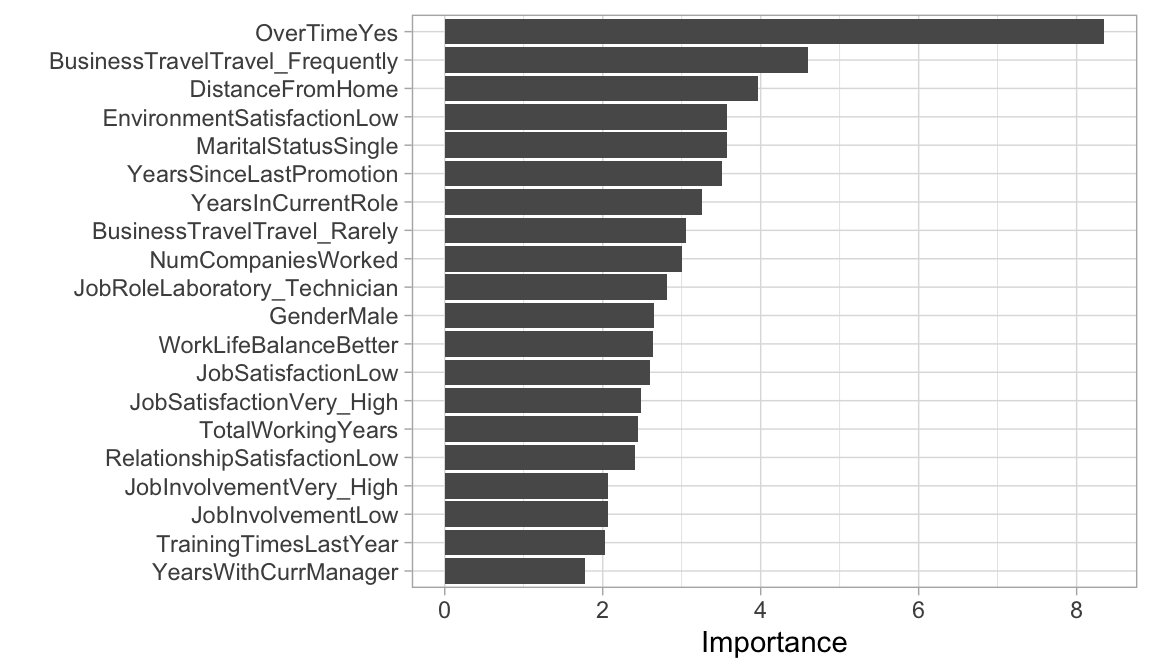
## 5 Fold5 roc_auc binary 0.845 Preprocessor1_Model111.9 Feature interpretation
Similar to linear regression, once our preferred logistic regression model is identified, we need to interpret how the features are influencing the results. As with normal linear regression models, variable importance for logistic regression models can be computed using the absolute value of the \(z\)-statistic for each coefficient. Using vip::vip() we can extract our top 20 influential variables. The following illustrates that for lr_fit4, working overtime is the most influential followed by the frequency of business travel and the distance from home that the employees office is.
11.10 Final thoughts
Logistic regression provides an alternative to linear regression for binary classification problems. However, similar to linear regression, logistic regression suffers from the many assumptions involved in the algorithm (i.e. linear relationship of the coefficient, multicollinearity). Moreover, often we have more than two classes to predict which is commonly referred to as multinomial classification. Although multinomial extensions of logistic regression exist, the assumptions made only increase and, often, the stability of the coefficient estimates (and therefore the accuracy) decrease. Future modules will discuss more advanced algorithms that provide a more natural and trustworthy approach to binary and multinomial classification prediction.
11.11 Exercises
Use the titanic.csv dataset available via Canvas for
these exercise questions. This dataset contains information on the fate
of 1,043 passengers on the fatal maiden voyage of the ocean liner
‘Titanic’. Our interest is in predicting whether or not a passenger
survived. Because the variable we want to predict is binary (survived =
Yes if the passenger survived and survived = No if they did not),
logistic regression is appropriate. For this session we’ll assess three
predictor variables: pclass, sex, and
age.
-
survived(dependent variable) = Yes if the passenger survived and No if they did not -
pclass(predictor variable) = the economic class of the passenger summarized as 1st, 2nd, 3rd, and Crew class. -
sex(predictor variable) = reported sex of the passenger (“male”, “female”) -
age(predictor variable) = age of passenger. Note that ages <1 are for infants.
Complete the following tasks:
- Using stratified sampling split the data into a training set and a test set. Use a 70/30 split (70% for the training data & 30% for the test set).
- Apply a logistic regression model using all predictor variables and perform a 10-fold cross validation procedure.
- What is the mean cross-validation generalization error?
- Identify the influence of the three predictor variables.