12 Lesson 4b: Regularized Regression
Linear models (LMs) provide a simple, yet effective, approach to predictive modeling. Moreover, when certain assumptions required by LMs are met (e.g., constant variance), the estimated coefficients are unbiased and, of all linear unbiased estimates, have the lowest variance. However, in today’s world, data sets being analyzed typically contain a large number of features. As the number of features grow, certain assumptions typically break down and these models tend to overfit the training data, causing our generalization error to increase. Regularization methods provide a means to constrain or regularize the estimated coefficients, which can reduce the variance and decrease the generalization error.
12.1 Learning objectives
By the end of this module you will know:
- Why reguralization is important.
- How to apply ridge, lasso, and elastic net regularized models.
- Extract and visualize the most influential features.
12.2 Prerequisites
12.3 Why regularize?
The easiest way to understand regularized regression is to explain how and why it is applied to ordinary least squares (OLS). The objective in OLS regression is to find the hyperplane (e.g., a straight line in two dimensions) that minimizes the sum of squared errors (SSE) between the observed and predicted response values (see Figure below). This means identifying the hyperplane that minimizes the grey lines, which measure the vertical distance between the observed (red dots) and predicted (blue line) response values.
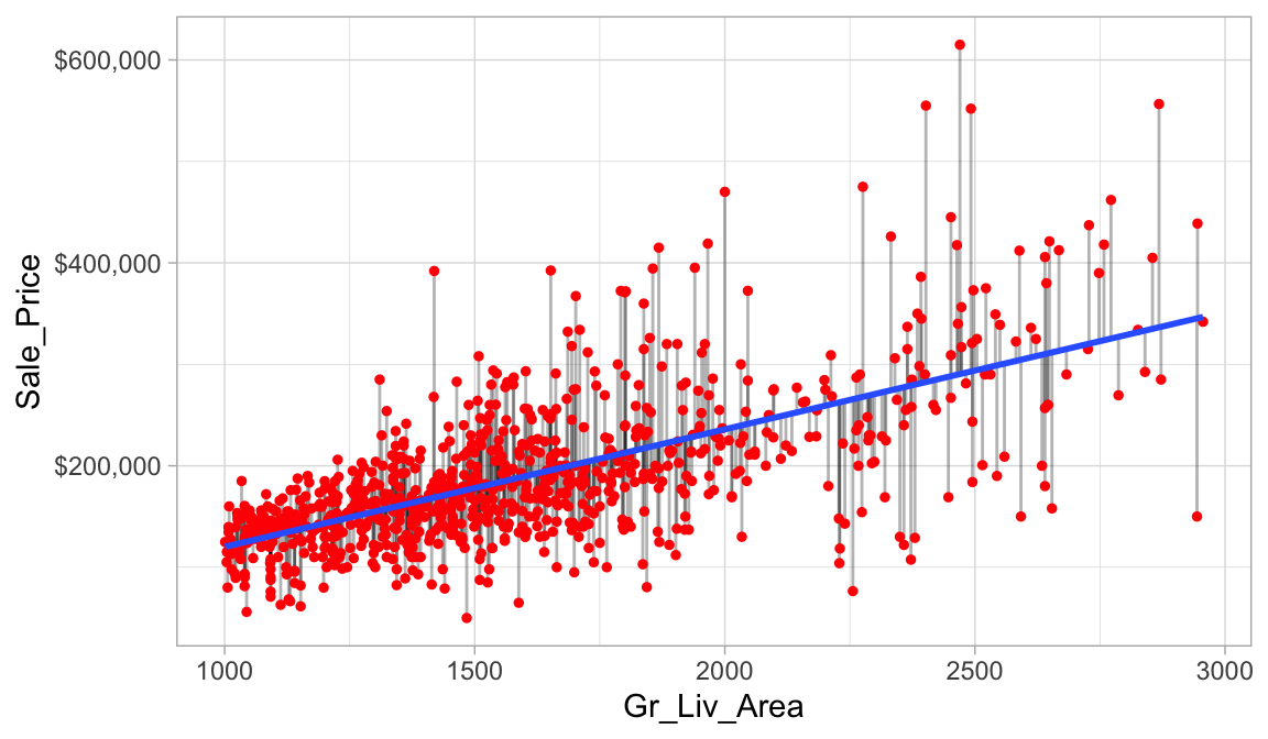
Figure 12.1: Figure: Fitted regression line using Ordinary Least Squares.
More formally, the objective function being minimized can be written as:
\[\begin{equation} \text{minimize} \left( SSE = \sum^n_{i=1} \left(y_i - \hat{y}_i\right)^2 \right) \end{equation}\]
Recall that we have use the following terms interchangably:
- Sum of squared errors (SSE)
- Residual sum of squares (RSS)
However, linear regression makes several strong assumptions that are often violated as we include more predictors in our model. Violation of these assumptions can lead to flawed interpretation of the coefficients and prediction results.
- Linear relationship: Linear regression assumes a linear relationship between the predictor and the response variable.
- More observations than predictors: Although not an issue with the Ames housing data, when the number of features exceeds the number of observations (\(p > n\)), the OLS estimates are not obtainable.
- No or little multicollinearity: Collinearity refers to the situation in which two or more predictor variables are closely related to one another. The presence of collinearity can pose problems in OLS, since it can be difficult to separate out the individual effects of collinear variables on the response. In fact, collinearity can cause predictor variables to appear as statistically insignificant when in fact they are significant. This obviously leads to an inaccurate interpretation of coefficients and makes it difficult to identify influential predictors.
There are other assumptions that ordinary least squares regression makes that are often violated with larger data sets.
Many real-life data sets, like those common to text mining and genomic studies are wide, meaning they contain a larger number of features (\(p > n\)). As p increases, we’re more likely to violate some of the OLS assumptions, which can cause poor model performance. Consequently, alternative algorithms should be considered.
Having a large number of features invites additional issues in using classic regression models. For one, having a large number of features makes the model much less interpretable. Additionally, when \(p > n\), there are many (in fact infinite) solutions to the OLS problem! In such cases, it is useful (and practical) to assume that a smaller subset of the features exhibit the strongest effects (something called the bet on sparsity principle (see Hastie, Tibshirani, and Wainwright 2015, 2).). For this reason, we sometimes prefer estimation techniques that incorporate feature selection. One approach to this is called hard thresholding feature selection, which includes many of the traditional linear model selection approaches like forward selection and backward elimination. These procedures, however, can be computationally inefficient, do not scale well, and treat a feature as either in or out of the model (hence the name hard thresholding). In contrast, a more modern approach, called soft thresholding, slowly pushes the effects of irrelevant features toward zero, and in some cases, will zero out entire coefficients. As will be demonstrated, this can result in more accurate models that are also easier to interpret.
With wide data (or data that exhibits multicollinearity), one alternative to OLS regression is to use regularized regression (also commonly referred to as penalized models or shrinkage methods as in J. Friedman, Hastie, and Tibshirani (2001) and Kuhn and Johnson (2013)) to constrain the total size of all the coefficient estimates. This constraint helps to reduce the magnitude and fluctuations of the coefficients and will reduce the variance of our model (at the expense of no longer being unbiased—a reasonable compromise).
The objective function of a regularized regression model is similar to OLS, albeit with a penalty term \(P\).
\[\begin{equation} \text{minimize} \left( SSE + P \right) \end{equation}\]
This penalty parameter constrains the size of the coefficients such that the only way the coefficients can increase is if we experience a comparable decrease in the sum of squared errors (SSE).
This concept generalizes to all GLM models (e.g., logistic and Poisson regression) and even some survival models. So far, we have been discussing OLS and the sum of squared errors loss function. However, different models within the GLM family have different loss functions (see Chapter 4 of J. Friedman, Hastie, and Tibshirani (2001)). Yet we can think of the penalty parameter all the same—it constrains the size of the coefficients such that the only way the coefficients can increase is if we experience a comparable decrease in the model’s loss function.
Regularized regression constrains the size of the predictor variable coefficients such that the only way the coefficients can increase is if we experience a comparable decrease in the model’s loss function.
Constraining coefficients actually creates more stable models, which can improve model performance and generalization.
There are three common penalty parameters we can implement:
- Ridge;
- Lasso (or LASSO);
- Elastic net (or ENET), which is a combination of ridge and lasso.
12.4 Ridge penalty
Ridge regression (Hoerl and Kennard 1970) controls the estimated coefficients by adding \(\lambda \sum^p_{j=1} \beta_j^2\) to the objective function.
\[\begin{equation} \text{minimize } \left( SSE + \lambda \sum^p_{j=1} \beta_j^2 \right) \end{equation}\]
The size of this penalty, referred to as \(L^2\) (or Euclidean) norm, can take on a wide range of values, which is controlled by the tuning parameter \(\lambda\). When \(\lambda = 0\) there is no effect and our objective function equals the normal OLS regression objective function of simply minimizing SSE. However, as \(\lambda \rightarrow \infty\), the penalty becomes large and forces the coefficients toward zero (but not all the way). This is illustrated below where exemplar coefficients have been regularized with \(\lambda\) ranging from 0 to over 8,000.
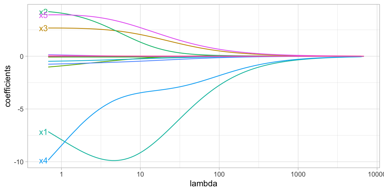
Figure 12.2: Figure: Ridge regression coefficients for 15 exemplar predictor variables as \(\lambda\) grows from \(0 \rightarrow \infty\). As \(\lambda\) grows larger, our coefficient magnitudes are more constrained.
Although these coefficients were scaled and centered prior to the analysis, you will notice that some are quite large when \(\lambda\) is near zero. Furthermore, you’ll notice that feature x1 has a large negative parameter that fluctuates until \(\lambda \approx 7\) where it then continuously shrinks toward zero. This is indicative of multicollinearity and likely illustrates that constraining our coefficients with \(\lambda > 7\) may reduce the variance, and therefore the error, in our predictions.
In essence, the ridge regression model pushes many of the correlated features toward each other rather than allowing for one to be wildly positive and the other wildly negative. In addition, many of the less-important features also get pushed toward zero. This helps to provide clarity in identifying the important signals in our data.
However, ridge regression does not perform feature selection and will retain all available features in the final model. Therefore, a ridge model is good if you believe there is a need to retain all features in your model yet reduce the noise that less influential variables may create (e.g., in smaller data sets with severe multicollinearity). If greater interpretation is necessary and many of the features are redundant or irrelevant then a lasso or elastic net penalty may be preferable.
12.5 Lasso penalty
The lasso (least absolute shrinkage and selection operator) penalty (Tibshirani 1996) is an alternative to the ridge penalty that requires only a small modification. The only difference is that we swap out the \(L^2\) norm for an \(L^1\) norm: \(\lambda \sum^p_{j=1} | \beta_j|\):
\[\begin{equation} \text{minimize } \left( SSE + \lambda \sum^p_{j=1} | \beta_j | \right) \end{equation}\]
Whereas the ridge penalty pushes variables to approximately but not equal to zero, the lasso penalty will actually push coefficients all the way to zero as illustrated in below. Switching to the lasso penalty not only improves the model but it also conducts automated feature selection.
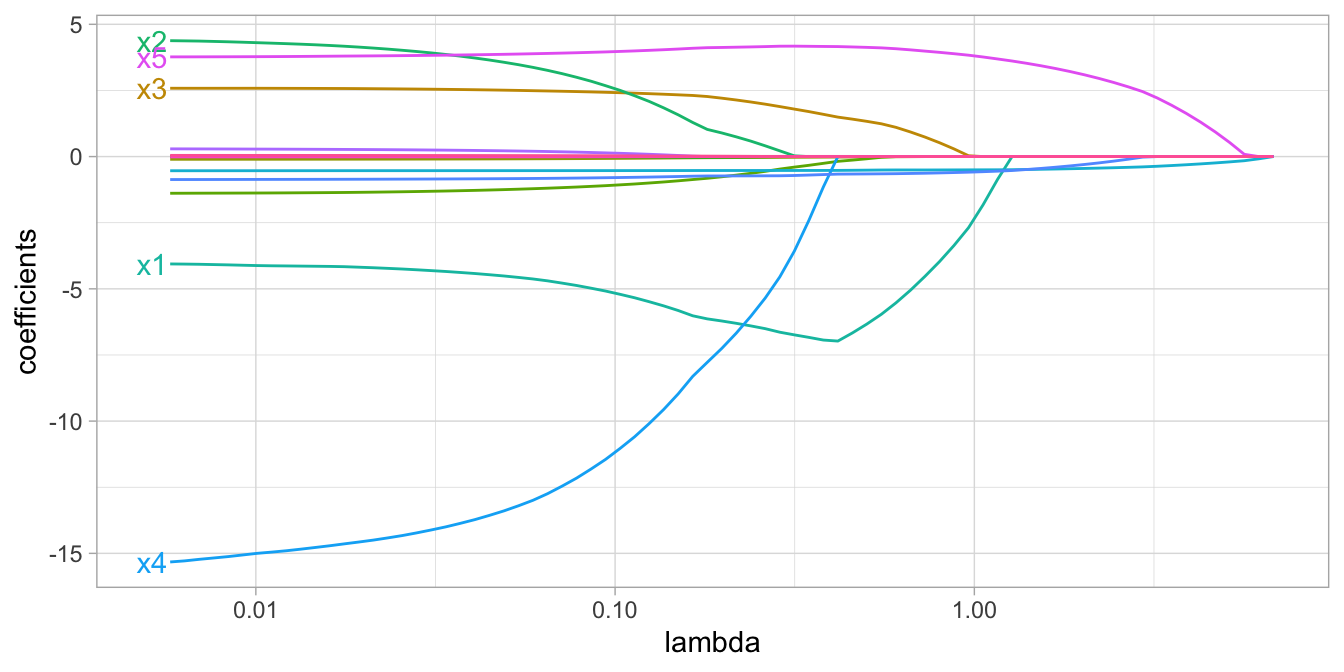
Figure 12.3: Figure: Lasso regression coefficients as \(\lambda\) grows from \(0 \rightarrow \infty\).
In the figure above we see that when \(\lambda < 0.01\) all 15 variables are included in the model, when \(\lambda \approx 0.5\) 9 variables are retained, and when \(log\left(\lambda\right) = 1\) only 5 variables are retained. Consequently, when a data set has many features, lasso can be used to identify and extract those features with the largest (and most consistent) signal.
12.6 Elastic nets
A generalization of the ridge and lasso penalties, called the elastic net (Zou and Hastie 2005), combines the two penalties:
\[\begin{equation} \text{minimize } \left( SSE + \lambda_1 \sum^p_{j=1} \beta_j^2 + \lambda_2 \sum^p_{j=1} | \beta_j | \right) \end{equation}\]
Although lasso models perform feature selection, when two strongly correlated features are pushed towards zero, one may be pushed fully to zero while the other remains in the model. Furthermore, the process of one being in and one being out is not very systematic. In contrast, the ridge regression penalty is a little more effective in systematically handling correlated features together. Consequently, the advantage of the elastic net penalty is that it enables effective regularization via the ridge penalty with the feature selection characteristics of the lasso penalty.
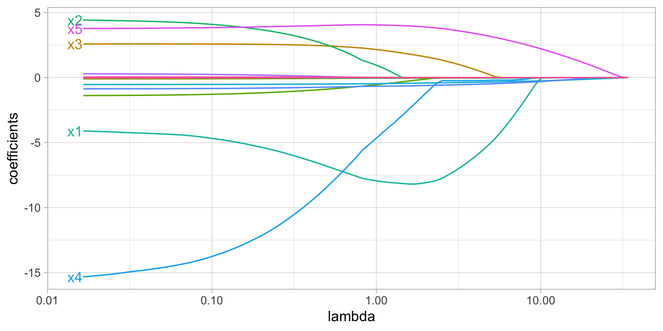
Figure 12.4: Figure: Elastic net coefficients as \(\lambda\) grows from \(0 \rightarrow \infty\).
12.7 Implementation
We will start by applying a simple ridge model. In this example we simplify and focus on only four features: Gr_Liv_Area, Year_Built, Garage_Cars, and Garage_Area. In this example we will apply a \(\lambda\) penalty parameter equal to 1.
Since regularized methods apply a penalty to the coefficients, we need to ensure our coefficients are on a common scale. If not, then predictors with naturally larger values (e.g., total square footage) will be penalized more than predictors with naturally smaller values (e.g., total number of rooms).
Takeaway - when using regularized regression models always standardize numeric features so they have mean 0 and standard deviation of 1.
To apply a regularized model we still use linear_reg() but we change the engine and provide some additional arguments. There are a few engines that allow us to apply regularized models but the most popular is glmnet. In R, the \(\lambda\) penalty parameter is represented by penalty and mixture controls the type of penalty (0 = ridge, 1 = lasso, and any value in between represents an elastic net).
# Step 1: create ridge model object
ridge_mod <- linear_reg(penalty = 1000, mixture = 0) %>%
  set_engine("glmnet")

# Step 2: create model & preprocessing recipe
model_recipe <- recipe(Sale_Price ~ ., data = ames_train) %>%
  step_normalize(all_numeric_predictors()) %>%
  step_dummy(all_nominal_predictors())

# Step 3: fit model workflow
ridge_fit <- workflow() %>%
  add_recipe(model_recipe) %>%
  add_model(ridge_mod) %>%
  fit(data = ames_train)

# Step 4: extract and tidy results
ridge_fit %>%
  extract_fit_parsnip() %>%
  tidy()
## # A tibble: 309 × 3
##    term           estimate penalty
##    <chr>             <dbl>   <dbl>
##  1 (Intercept)     154704.    1000
##  2 Lot_Frontage      -841.    1000
##  3 Lot_Area          4067.    1000
##  4 Year_Built        4962.    1000
##  5 Year_Remod_Add    2876.    1000
##  6 Mas_Vnr_Area      3940.    1000
##  7 BsmtFin_SF_1      -957.    1000
##  8 BsmtFin_SF_2       597.    1000
##  9 Bsmt_Unf_SF      -2925.    1000
## 10 Total_Bsmt_SF     5941.    1000
## # ℹ 299 more rows
Using tidy() on our fit workflow provides the regularized coefficients. Note that these coefficients are interpreted differently than in previous modules since we standardized our features.
Since our features are standardized to mean = 0 and standard deviation = 1, we interpret the coefficients as…
For every 1 standard deviation above the mean
Year_Built, the average predicted Sale_Price
increases by $4,962.
How well does our model perform, let’s use a 5-fold cross validation procedure to compute our generalization error:
set.seed(123)
kfolds <- vfold_cv(ames_train, v = 5, strata = Sale_Price)

workflow() %>%
   add_recipe(model_recipe) %>%
   add_model(ridge_mod) %>%
   fit_resamples(kfolds) %>%
   collect_metrics() %>%
   filter(.metric == 'rmse')
## # A tibble: 1 × 6
##   .metric .estimator   mean     n std_err .config
##   <chr>   <chr>       <dbl> <int>   <dbl> <chr>
## 1 rmse    standard   31373.     5   3012. Preprocessor1_Model1
12.7.1 Knowledge check
Using the boston.csv data provided via Canvas fill in
the blanks to…
- create train and test splits,
- create ridge model object using \(\lambda = 5000\),
-
create model (our response variable
cmedvshould be a function of all predictor variables) & preprocessing recipe where you standardize all predictor variables, - create 5-fold resampling object stratified on the response variable,
- fit model across resampling object and compute the cross validation RMSE.
# Step 1: create train and test splits
set.seed(123)  # for reproducibility
split  <- initial_split(_______, prop = 0.7, strata = "cmedv")
boston_train  <- training(split)
boston_test   <- testing(split)

# Step 2: create ridge model object
ridge_mod <- linear_reg(penalty = ____, mixture = __) %>%
  set_engine("glmnet")

# Step 3: create model & preprocessing recipe
model_recipe <- recipe(cmedv ~ ., data = _______) %>%
  step_normalize(________)

# Step 4: create 5-fold resampling object
set.seed(123)
kfolds <- vfold_cv(______, v = 5, strata = _______)

# Step 5: fit model across resampling object and collect results
workflow() %>%
   add_recipe(________) %>%
   add_model(________) %>%
   fit_resamples(________) %>%
   collect_metrics() %>%
   filter(.metric == 'rmse')
12.8 Tuning our model
It’s important to note that there are two main parameters that we, the data scientists, control setting the values for:
mixture: the type of regularization (ridge, lasso, elastic net) we want to apply and,penalty: the strength of the regularization parameter, which we referred to as \(\lambda\) in earlier sections.
These parameters can be thought of as “the knobs to twiddle”4 and we often refer to them as hyperparameters.
Hyperparameters (aka tuning parameters) are parameters that we can use to control the complexity of machine learning algorithms. Not all algorithms have hyperparameters (e.g., ordinary least squares); however, more advanced algorithms have at least one or more.
The proper setting of these hyperparameters is often dependent on the data and problem at hand and cannot always be estimated by the training data alone. Consequently, we often go through iterations of testing out different values to determine which hyperparameter settings provide the optimal result.
In the next module we’ll see how we can automate the hyperparameter tuning process. For now, we’ll simply take a manual approach.
12.8.1 Tuning regularization strength
First, we’ll asses how the regularization strength impacts the performance of our model. In the two examples that follow we will use all the features in our Ames housing data; however, we’ll stick to the basic preprocessing of standardizing our numeric features and dummy encoding our categorical features.
For both models we still use a ridge model (mixture = 0) but we assess two different values for \(\lambda\) (penalty). Note how increasing the penalty leads to a lower RMSE.
Having the larger penalty will not always lead to a
lower RMSE, it just happens to be the case for this data set. This is
likely because we have high collinearity across our predictors so a
larger penalty is helping to constrain the coefficients and
make them more stable.
####################################
# Ridge model with penalty = 10000 #
####################################

# create linear model object
ridge_mod <- linear_reg(penalty = 10000, mixture = 0) %>%
  set_engine("glmnet")

workflow() %>%
   add_recipe(model_recipe) %>%
   add_model(ridge_mod) %>%
   fit_resamples(kfolds) %>%
   collect_metrics() %>%
   filter(.metric == 'rmse')
## # A tibble: 1 × 6
##   .metric .estimator   mean     n std_err .config
##   <chr>   <chr>       <dbl> <int>   <dbl> <chr>
## 1 rmse    standard   30999.     5   2816. Preprocessor1_Model1
####################################
# Ridge model with penalty = 20000 #
####################################
# create linear model object
ridge_mod <- linear_reg(penalty = 20000, mixture = 0) %>%
set_engine("glmnet")
ridge_fit <- workflow() %>%
add_recipe(model_recipe) %>%
add_model(ridge_mod) %>%
fit_resamples(kfolds)
collect_metrics(ridge_fit) %>%
filter(.metric == 'rmse')
## # A tibble: 1 × 6
## .metric .estimator mean n std_err .config
## <chr> <chr> <dbl> <int> <dbl> <chr>
## 1 rmse standard 30678. 5 2598. Preprocessor1_Model112.8.2 Tuning regularization type
We should also assess the type of regularization we want to apply (i.e. Ridge, Lasso, Elastic Net). It is not always definitive which type of regularization will perform best; however, often Ridge or some combination of both \(L^1\) and \(L^2\) (elastic net) performs best while Lasso is more useful if we desire to eliminate noisy features altogether.
The following uses the same penalty as we did previously but changes the regularization type to Lasso (mixture = 1) and Elastic Net with a 50-50 mixture of \(L^1\) and \(L^2\) (mixture = 0.5).
####################################
# Lasso model with penalty = 20000 #
####################################

# create linear model object
lasso_mod <- linear_reg(penalty = 20000, mixture = 1) %>%
  set_engine("glmnet")

lasso_fit <- workflow() %>%
   add_recipe(model_recipe) %>%
   add_model(lasso_mod) %>%
   fit_resamples(kfolds)

collect_metrics(lasso_fit) %>%
   filter(.metric == 'rmse')
## # A tibble: 1 × 6
##   .metric .estimator   mean     n std_err .config
##   <chr>   <chr>       <dbl> <int>   <dbl> <chr>
## 1 rmse    standard   48675.     5   2034. Preprocessor1_Model1
##########################################
# Elastic net model with penalty = 20000 #
##########################################
# create linear model object
elastic_mod <- linear_reg(penalty = 20000, mixture = 0.5) %>%
set_engine("glmnet")
elastic_fit <- workflow() %>%
add_recipe(model_recipe) %>%
add_model(elastic_mod) %>%
fit_resamples(kfolds)
collect_metrics(elastic_fit) %>%
filter(.metric == 'rmse')
## # A tibble: 1 × 6
## .metric .estimator mean n std_err .config
## <chr> <chr> <dbl> <int> <dbl> <chr>
## 1 rmse standard 39730. 5 2433. Preprocessor1_Model1We see that in both cases the 5-fold cross validation error is higher than the Ridge model.
12.8.3 Tuning regularization type & strength
Unfortunately, using the same penalty value across the different models rarely works to find the optimal model. Not only do we need to tune the regularization type (Ridge, Lasso, Elastic Net), but we also need to tune the penalty value for each regularization type.
This becomes far more tedious and we’d rather not manually test out many values. In the next module we’ll discuss how we can automate the tuning process to find optimal results.
12.8.4 Knowledge check
Using the same boston training data as in the previous
knowledge check, fill in the blanks to test a variety of values for…
- The type of regularization. Try a Lasso model versus an elastic net.
- The value of the penalty. Does a higher or lower penalty improve performance?
# Step 2: create ridge model object
glm_mod <- linear_reg(penalty = ____, mixture = __) %>%
  set_engine("glmnet")

# Step 3: create model & preprocessing recipe
model_recipe <- recipe(cmedv ~ ., data = boston_train) %>%
  step_normalize(all_numeric_predictors())

# Step 4: create 5-fold resampling object
set.seed(123)
kfolds <- vfold_cv(boston_train, v = 5, strata = cmedv)

# Step 5: fit model across resampling object and collect results
workflow() %>%
   add_recipe(model_recipe) %>%
   add_model(glm_mod) %>%
   fit_resamples(kfolds) %>%
   collect_metrics() %>%
   filter(.metric == 'rmse')
12.9 Feature importance
For regularized models, importance is determined by magnitude of the standardized coefficients. Recall that ridge, lasso, and elastic net models push non-influential features to zero (or near zero). Consequently, very small coefficient values represent features that are not very important while very large coefficient values (whether negative or positive) represent very important features.
We’ll check out the ridge model since that model performed best. We just need to fit a final model across all the training data, extract that final fit from the workflow object, and then use the vip package to visualize the variable importance scores for the top 20 features:
final_fit <- workflow() %>%
   add_recipe(model_recipe) %>%
   add_model(ridge_mod) %>%
   fit(data = ames_train)

final_fit %>%
   extract_fit_parsnip() %>%
   vip(num_features = 20, geom = "point")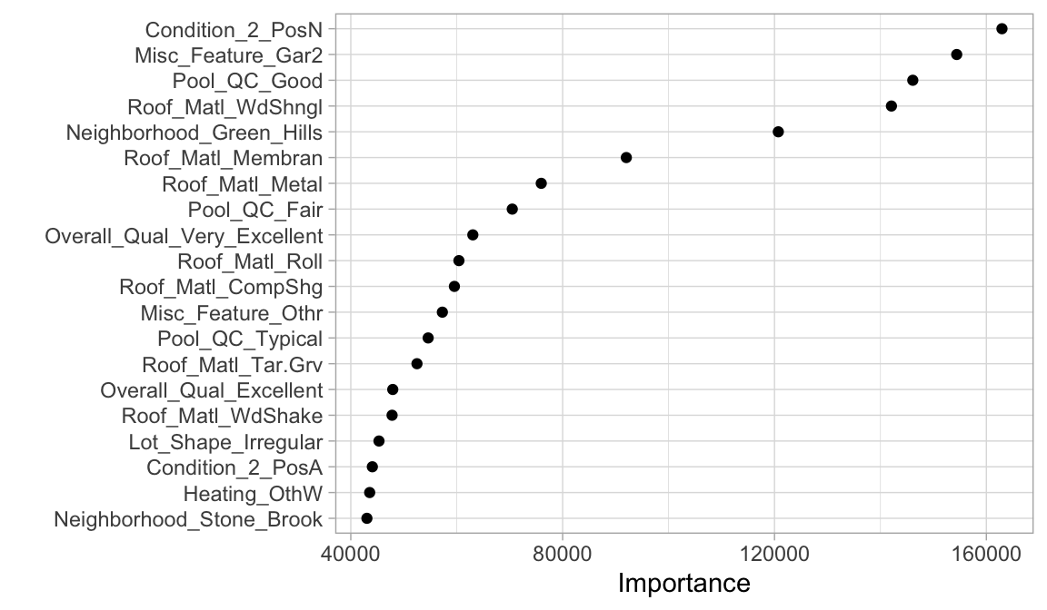
12.10 Classification problems
We saw that we can apply regularization to a regression problem but we can also do the same for classification problems. The following applies the same procedures we used above but for the kernlab::spam data.
library(kernlab)
data(spam)

# Step 1: create train and test splits
set.seed(123)  # for reproducibility
split  <- initial_split(spam, prop = 0.7, strata = "type")
spam_train  <- training(split)
spam_test   <- testing(split)

# Step 2: create ridge model object
ridge_mod <- logistic_reg(penalty = 100, mixture = 0) %>%
   set_engine("glmnet") %>%
   set_mode("classification")

# Step 3: create model & preprocessing recipe
model_recipe <- recipe(type ~ ., data = spam_train) %>%
  step_normalize(all_numeric_predictors())

# Step 4: create workflow object to combine the recipe & model
spam_wf <- workflow() %>%
   add_recipe(model_recipe) %>%
   add_model(ridge_mod)

# Step 5: fit model across resampling object and collect results
set.seed(123)
kfolds <- vfold_cv(spam_train, v = 5, strata = "type")

spam_wf %>%
   fit_resamples(kfolds) %>%
   collect_metrics()
## # A tibble: 3 × 6
##   .metric     .estimator  mean     n   std_err .config
##   <chr>       <chr>      <dbl> <int>     <dbl> <chr>
## 1 accuracy    binary     0.606     5 0.000197  Preprocessor1_Model1
## 2 brier_class binary     0.237     5 0.0000497 Preprocessor1_Model1
## 3 roc_auc     binary     0.946     5 0.00274   Preprocessor1_Model1
# Step 6: Fit final model on all training data
final_fit <- spam_wf %>%
fit(data = spam_train)
# Step 7: Assess top 20 most influential features
final_fit %>%
extract_fit_parsnip() %>%
vip(num_features = 20, geom = "point")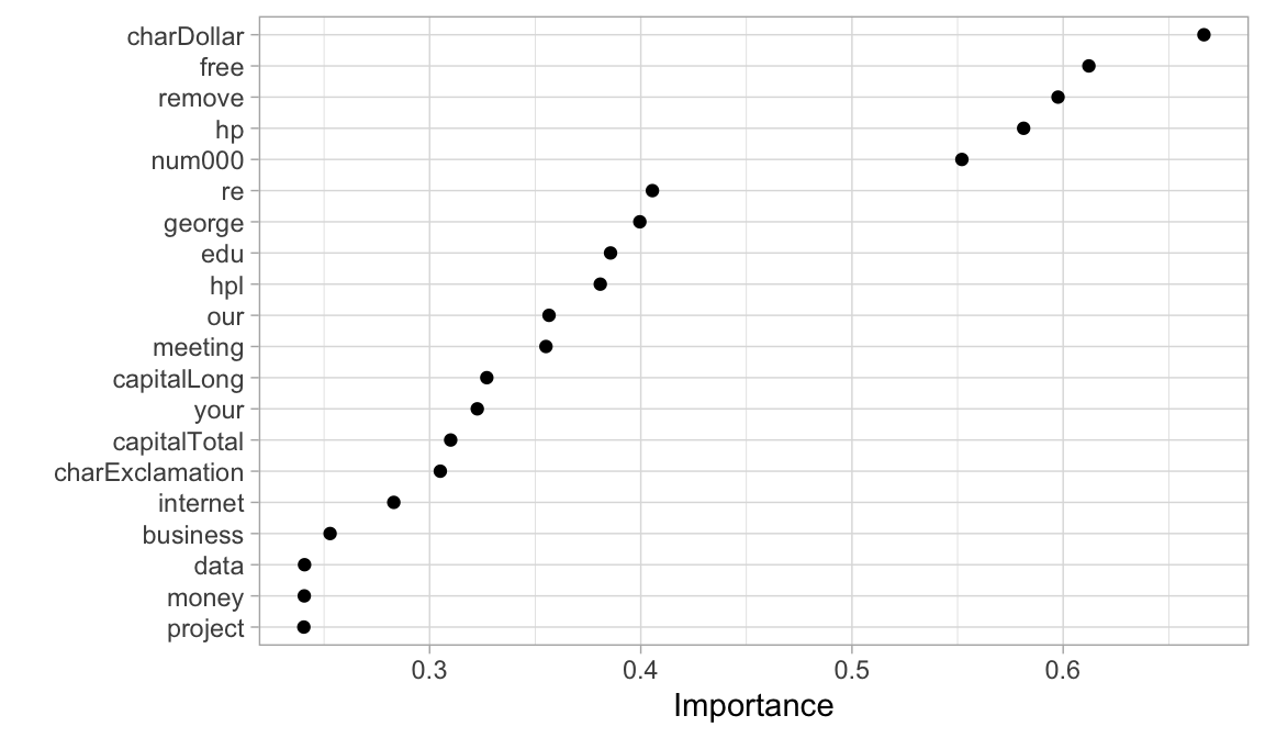
12.11 Final thoughts
Regularized regression provides many great benefits over traditional GLMs when applied to large data sets with lots of features. It provides a great option for handling the \(n > p\) problem, helps minimize the impact of multicollinearity, and can perform automated feature selection. It also has relatively few hyperparameters which makes them easy to tune, computationally efficient compared to other algorithms discussed in later modules, and memory efficient.
However, similar to GLMs, they are not robust to outliers in both the feature and target. Also, regularized regression models still assume a monotonic linear relationship (always increasing or decreasing in a linear fashion). It is also up to the analyst whether or not to include specific interaction effects.
12.12 Exercises
Recall the Advertising.csv dataset we used in the Resampling
lesson. Use this same data (available via Canvas) to…
- Split the data into 70-30 training-test sets.
-
Apply a ridge model with
Salesbeing the response variable. Perform a cross-validation procedure and test the model across various penalty parameter values. Which penalty parameter value resulted in the lowest RMSE? - Repeat #2 but changing the regularization type to Lasso and Elastic net. Which regularization type results in the lowest RMSE?
- Using the best model from those that you tested out in #2 and #3, plot the feature importance. Which feature is most influential? Which is least influential?