9 Lesson 3b: Resampling
The last several lessons gave you a good introduction to building predictive models using the tidymodels construct. And as we trained our models we evaluated their performance on the test set, which we called the generalization error. However, the approach we’ve taken thus far to evaluate the generalization error can have some pitfalls. This lesson is going to go deeper into the idea of model evaluation and we’ll discuss how to incorporate resampling procedures to give you a more robust assessment of model performance.
9.1 Learning objectives
By the end of this lesson you will be able to:
- Explain the reasoning for resampling procedures and when/why we should incorporate them into our ML workflow.
- Implement k-fold cross-validation procedures for more robust model evaluation.
- Implement bootstrap resampling procedures for more robust model evaluation.
9.2 Prerequisites
This lesson leverages the following packages and data.
Let’s go ahead and create our train-test split:
9.3 Resampling & cross-validation
In the previous lessons we split our data into a train and test set and we assessed the performance of our model on the test set. If we use a little feature engineering to take care of novel categorical levels, we see that our generalization RMSE based on the test set is $26,144.
mlr_recipe <- recipe(Sale_Price ~ ., data = ames_train) %>%
   step_other(all_nominal_predictors(), threshold = 0.02, other = "other")

mlr_wflow <- workflow() %>%
  add_model(linear_reg()) %>%
  add_recipe(mlr_recipe)

mlr_fit <- mlr_wflow %>%
   fit(data = ames_train)

mlr_fit %>%
   predict(ames_test) %>%
   bind_cols(ames_test %>% select(Sale_Price)) %>%
   rmse(truth = Sale_Price, estimate = .pred)
## # A tibble: 1 × 3
##   .metric .estimator .estimate
##   <chr>   <chr>          <dbl>
## 1 rmse    standard      26144.
Unfortunately, there are a few pitfalls to this approach:
- If our dataset is small, a single test set may not provide realistic expectations of our model’s performance on unseen data.
- A single test set does not provide us any insight on variability of our model’s performance.
- Using our test set to drive our model building process can bias our results via data leakage. Basically, the more we use the test data to assess various model performances, the less likely the test data is behaving like true, unseen data.
It is critical that the test set not be used prior to selecting your final model. Assessing results on the test set prior to final model selection biases the model selection process since the testing data will have become part of the model development process.
Resampling methods provide an alternative approach by allowing us to repeatedly fit a model of interest to parts of the training data and test its performance on other parts of the training data.
Figure 9.1: Illustration of resampling. (Kuhn, Max n.d.)
This allows us to train and validate our model entirely on the training data and not touch the test data until we have selected a final “optimal” model.
The two most commonly used resampling methods include k-fold cross-validation and bootstrap sampling.
9.4 K-fold cross-validation
Cross-validation consists of repeating the procedure such that the training and testing sets are different each time. Generalization performance metrics are collected for each repetition and then aggregated. As a result we can get an estimate of the variability of the model’s generalization performance.
k-fold cross-validation (aka k-fold CV) is a resampling method that randomly divides the training data into k groups (aka folds) of approximately equal size.
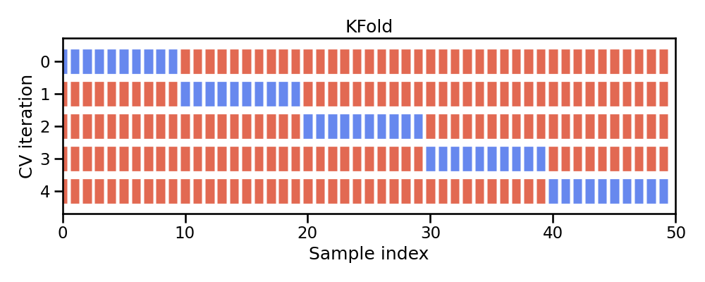
Figure 9.2: Illustration of k-fold sampling across a data sets index.
The model is fit on \(k-1\) folds and then the remaining fold is used to compute model performance. This procedure is repeated k times; each time, a different fold is treated as the validation set. Consequently, with k-fold CV, every observation in the training data will be held out one time to be included in the assessment/validation set. This process results in k estimates of the generalization error (say \(\epsilon_1, \epsilon_2, \dots, \epsilon_k\)). Thus, the k-fold CV estimate is computed by averaging the k test errors, providing us with an approximation of the error we might expect on unseen data.
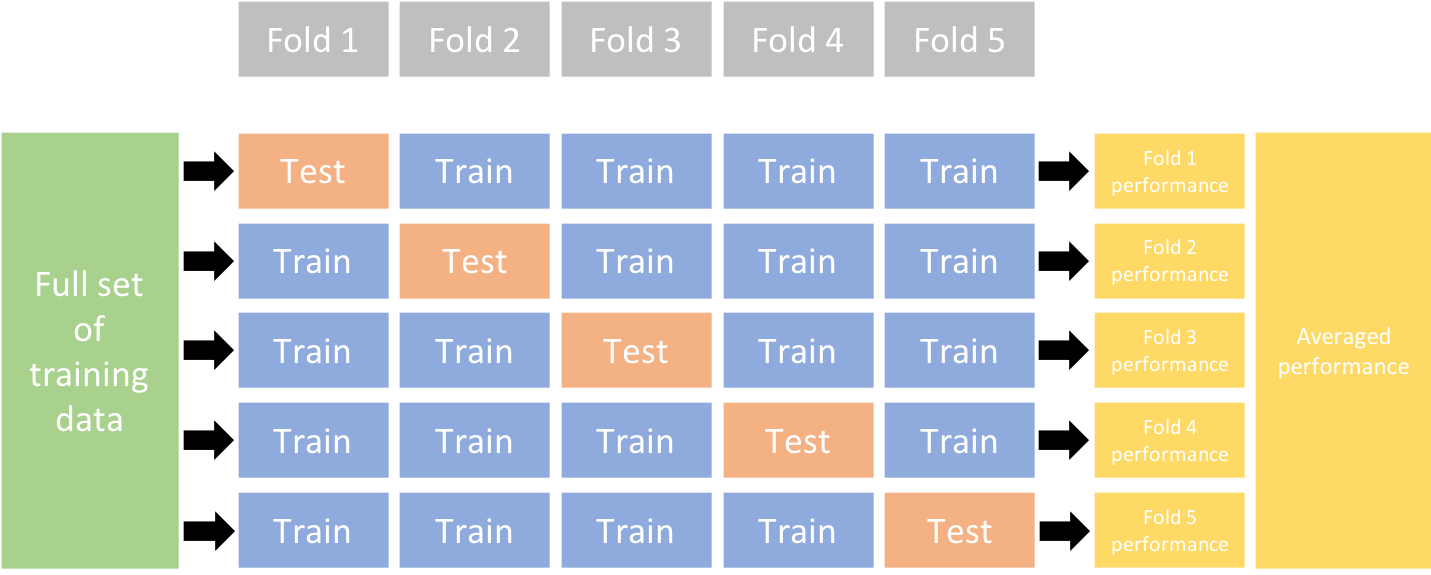
Figure 9.3: Illustration of a 5-fold cross validation procedure.
In practice, one typically uses k=5 or k=10. There is no formal rule as to the size of k; however, as k gets larger, the difference between the estimated performance and the true performance to be seen on the test set will decrease.
To implement k-fold CV we first make a resampling object. In this example we create a 10-fold resampling object.
We can now create our multiple linear regression workflow object as we did previously and fit our model across our 10-folds; we just use fit_resamples() rather than fit().
mlr_recipe <- recipe(Sale_Price ~ ., data = ames_train) %>%
   step_other(all_nominal_predictors(), threshold = 0.03, other = "other")

mlr_wflow <- workflow() %>%
  add_model(linear_reg()) %>%
  add_recipe(mlr_recipe)

# fit our model across the 10-fold CV
mlr_fit_cv <- mlr_wflow %>%
   fit_resamples(kfolds)
We can then get our average 10-fold cross validation error with collect_metrics():
collect_metrics(mlr_fit_cv)
## # A tibble: 2 × 6
##   .metric .estimator      mean     n   std_err .config
##   <chr>   <chr>          <dbl> <int>     <dbl> <chr>
## 1 rmse    standard   32547.       10 2455.     Preprocessor1_Model1
## 2 rsq     standard       0.839    10    0.0237 Preprocessor1_Model1
If we want to see the model evaluation metric (i.e. RMSE) for each fold we just need to include summarize = FALSE.
collect_metrics(mlr_fit_cv, summarize = FALSE) %>%
   filter(.metric == 'rmse')
## # A tibble: 10 × 5
##    id     .metric .estimator .estimate .config
##    <chr>  <chr>   <chr>          <dbl> <chr>
##  1 Fold01 rmse    standard      36485. Preprocessor1_Model1
##  2 Fold02 rmse    standard      37722. Preprocessor1_Model1
##  3 Fold03 rmse    standard      47136. Preprocessor1_Model1
##  4 Fold04 rmse    standard      24794. Preprocessor1_Model1
##  5 Fold05 rmse    standard      27203. Preprocessor1_Model1
##  6 Fold06 rmse    standard      28096. Preprocessor1_Model1
##  7 Fold07 rmse    standard      22781. Preprocessor1_Model1
##  8 Fold08 rmse    standard      36901. Preprocessor1_Model1
##  9 Fold09 rmse    standard      26510. Preprocessor1_Model1
## 10 Fold10 rmse    standard      37841. Preprocessor1_Model1
If we compare these results to our previous generalization error based on the test set, we see some differences. We now see that our average generalization RMSE across the ten holdout sets is $32,547 and individual validation set RMSEs range from $24,794 - $47,136. This provides us a little more robust expectations around how our model will perform on future unseen data. And it actually shows us that our single test set RMSE may have been biased and too optimistic!
One other item to note - often, people assume that when creating the k-folds that R just selects the first n observations to be the first fold, the next n observations to be in the second fold, etc. However, this is not the case. Rather, R will randomly assign observations to each fold but will also ensure that each observation is only assigned to a single fold for validation purposes. The following illustrates a 10-fold cross validation on a dataset with 32 observations. Each observation is used once for validation and nine times for training.
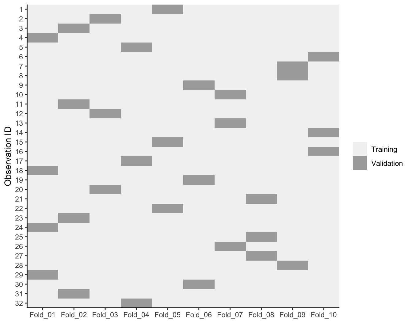
Figure 9.4: 10-fold cross validation on 32 observations. Each observation is used once for validation and nine times for training.
9.4.1 Knowledge check
Using the boston.csv data…
- Fill in the blanks to create a multiple linear regression model using all predictors (without any feature engineering); however, rather than computing the generalization error using the test data, apply 10-fold cross-validation.
- What is the average cross-validation RMSE?
- What is the range of cross-validation RMSE values across all ten folds?
# 1. Create a k-fold object
set.seed(123)
kfolds <- vfold_cv(______, v = __, strata = cmedv)

# 2. Create our workflow object
mlr_recipe <- recipe(cmedv ~ ___, data = boston_train)

mlr_wflow <- workflow() %>%
  add_model(______) %>%
  add_recipe(______)

# 3. Fit our model on the k-fold object
mlr_fit_cv <- mlr_wflow %>%
   fit_______(______)

# 4. Assess our average cross validation error
collect_______(______)
9.5 Bootstrap resampling
A bootstrap sample is a random sample of the data taken with replacement (Efron and Tibshirani 1986). This means that, after a data point is selected for inclusion in the subset, it’s still available for further selection. A bootstrap sample is the same size as the original data set from which it was constructed. Figure 9.5 provides a schematic of bootstrap sampling where each bootstrap sample contains 12 observations just as in the original data set. Furthermore, bootstrap sampling will contain approximately the same distribution of values (represented by colors) as the original data set.
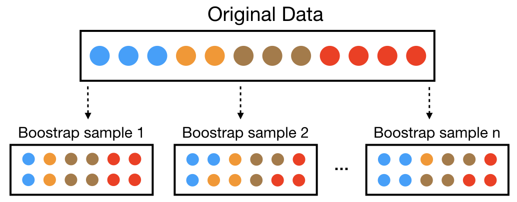
Figure 9.5: Illustration of the bootstrapping process.
Since samples are drawn with replacement, each bootstrap sample is likely to contain duplicate values. In fact, on average, \(\approx 63.21\)% of the original sample ends up in any particular bootstrap sample. The original observations not contained in a particular bootstrap sample are considered out-of-bag (OOB). When bootstrapping, a model can be built on the selected samples and validated on the OOB samples; this is often done, for example, in random forests (which we’ll discuss in a later module).
Since observations are replicated in bootstrapping, there tends to be less variability in the error measure compared with k-fold CV (Efron 1983). However, this can also increase the bias of your error estimate (we’ll discuss the concept of bias versus variance in a future module). This can be problematic with smaller data sets; however, for most average-to-large data sets (say \(n \geq 1,000\)) this concern is often negligible.
Figure 9.6 compares bootstrapping to 10-fold CV on a small data set with \(n = 32\) observations. A thorough introduction to the bootstrap and its use in R is provided in Davison, Hinkley, et al. (1997).
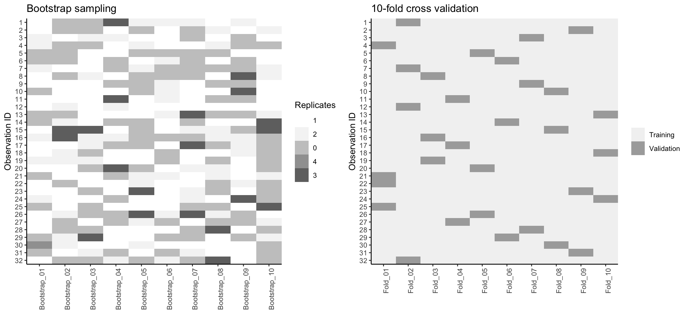
Figure 9.6: Bootstrap sampling (left) versus 10-fold cross validation (right) on 32 observations. For bootstrap sampling, the observations that have zero replications (white) are the out-of-bag observations used for validation.
We can create bootstrap samples easily with bootstraps(), as illustrated in the code chunk below.
Once we’ve created our bootstrap samples we can reuse the same mlr_wflow object we created earlier and refit it with the bootstrap samples. Our results again show that our average resampling RMSE is $38,765 – again, much higher than the single test set RMSE we obtained previously.
# fit our model across the bootstrapped samples
mlr_fit_bs <- mlr_wflow %>%
   fit_resamples(bs_samples)


collect_metrics(mlr_fit_bs)
## # A tibble: 2 × 6
##   .metric .estimator      mean     n   std_err .config
##   <chr>   <chr>          <dbl> <int>     <dbl> <chr>
## 1 rmse    standard   38765.        9 1885.     Preprocessor1_Model1
## 2 rsq     standard       0.780     9    0.0157 Preprocessor1_Model1
Bootstrapping is, typically, more of an internal resampling procedure that is naturally built into certain ML algorithms. This will become more apparent in later modules where we discuss bagging and random forests.
9.5.1 Knowledge check
Using the boston.csv data…
- Fill in the blanks to create a multiple linear regression model using all predictors (without any feature engineering); however, apply 10 bootstrap samples to compute the cross-validation RMSE.
- What is the average cross-validation RMSE?
- What is the range of cross-validation RMSE values across all ten folds?
- How do the results compare to the 10-fold cross validation you performed earlier?
# 1. Create a bootstrap object
set.seed(123)
bs_samples <- bootstraps(______, times = ___, strata = ____) #<<

# 2. Create our workflow object
mlr_recipe <- recipe(____ ~ __, data = boston_train)

mlr_wflow <- workflow() %>%
  add_model(______) %>%
  add_recipe(______)

# 3. Fit our model on the bootstrap object
mlr_fit_cv <- mlr_wflow %>%
   fit_______(______)

# 4. Assess our average cross validation error
______
9.6 Alternative methods
It is important to note that there are other useful resampling procedures. If you’re working with time-series specific data then you will want to incorporate rolling origin and other time series resampling procedures. Hyndman and Athanasopoulos (2018) is the dominant, R-focused, time series resource3.
Additionally, Efron (1983) developed the “632 method” and Efron and Tibshirani (1997) discuss the “632+ method”; both approaches seek to minimize biases experienced with bootstrapping on smaller data sets.
Other methods exist but K-fold cross validation and bootstrapping are the dominant methods used and are often sufficient.
9.7 Exercises
Use the Advertising.csv data to complete the following tasks. The
Advertising.csv data contains three predictor variables -
TV, Radio, and Newspaper, which
represents a companies advertising budget for these respective mediums
across 200 metropolitan markets. It also contains the response variable
- Sales, which represents the total sales in thousands of
units for a given product.
- Split the data into 70-30 training-test sets.
-
Using 10-fold cross-validation, create a multiple linear regression
model where
Salesis a function of all three predictors (without any feature engineering).- What is the average cross-validation RMSE?
- What is the range of cross-validation RMSE values across all ten folds?
-
Using boostrap resampling with 10 bootstrap samples, create a
multiple linear regression model where
Salesis a function of all three predictors (without any feature engineering).- What is the average bootstrap RMSE?
- What is the range of bootstrap RMSE values across all ten bootstrap samples?
References
See their open source book at https://www.otexts.org/fpp2↩︎