14 Lesson 5a: Hyperparameter Tuning

We learned in the last lesson that hyperparameters (aka tuning parameters) are parameters that we can use to control the complexity of machine learning algorithms. The proper setting of these hyperparameters is often dependent on the data and problem at hand and cannot always be estimated by the training data alone. Consequently, we often go through iterations of testing out different values to determine which hyperparameter settings provide the optimal result. As we add more hyperparameters, this becomes quite tedious to do manually so in this lesson we’ll learn how we can automate the tuning process to find the optimal (or near-optimal) settings for hyperparameters.

14.1 Learning objectives

By the end of this module you will:

• Be able to explain the two components that make up prediction errors.
• Understand why hyperparameter tuning is an essential part of the machine learning process.
• Apply efficient and effective hyperparameter tuning with Tidymodels.

14.2 Prerequisites

# Helper packages
library(tidyverse) # for data wrangling & plotting

# Modeling packages
library(tidymodels)

# Model interpretability packages
library(vip)      # variable importance

# Stratified sampling with the rsample package
ames <- AmesHousing::make_ames()
set.seed(123)  # for reproducibility
split  <- initial_split(ames, prop = 0.7, strata = "Sale_Price")
ames_train  <- training(split)
ames_test   <- testing(split)

14.3 Bias-variance tradeoff

Prediction errors can be decomposed into two important subcomponents: error due to “bias” and error due to “variance”. There is often a tradeoff between a model’s ability to minimize bias and variance. Understanding how different sources of error lead to bias and variance helps us improve the data fitting process resulting in more accurate models.

14.3.1 Bias

Bias is the difference between the expected (or average) prediction of our model and the correct value which we are trying to predict. It measures how far off in general a model’s predictions are from the correct value, which provides a sense of how well a model can conform to the underlying structure of the data. Figure 14.1 illustrates an example where the polynomial model does not capture the underlying structure well. Linear models are classical examples of high bias models as they are less flexible and rarely capture non-linear, non-monotonic relationships.

We can think of models with high bias as underfitting to the true patterns and relationships in our data. This is often because high bias models either oversimplify these relationships or are constrained in a way that cannot adequately form to the true, complex relationship that exists. These models tend to lead to high error on training and test data.

We also need to think of bias-variance in relation to resampling. Models with high bias are rarely affected by the noise introduced by resampling. If a model has high bias, it will have consistency in its resampling performance as illustrated below:

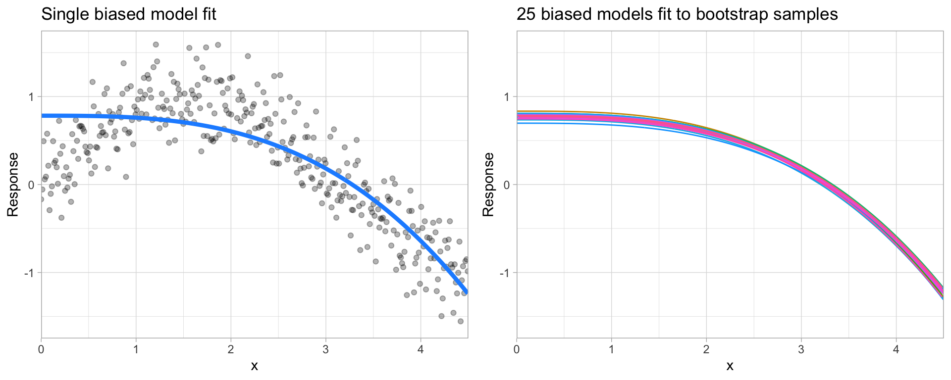
Figure 14.1: A biased polynomial model fit to a single data set does not capture the underlying non-linear, non-monotonic data structure (left). Models fit to 25 bootstrapped replicates of the data are underterred by the noise and generates similar, yet still biased, predictions (right).

14.3.2 Variance

On the other hand, error due to variance is defined as the variability of a model prediction for a given data point. Many models (e.g., k-nearest neighbor, decision trees, gradient boosting machines) are very adaptable and offer extreme flexibility in the patterns that they can fit to. However, these models offer their own problems as they run the risk of overfitting to the training data. Although you may achieve very good performance on your training data, the model will not automatically generalize well to unseen data.

Models with high variance can be very adaptable and will conform very well to the patterns and relationships in the training data. In fact, these models will try to overfit to patterns and relationships in the training data so much that they are overly personalized to the training data and will not generalize well to data which it hasn’t seen before. As a result, such models perform very well on training data but have high error rates on test data.

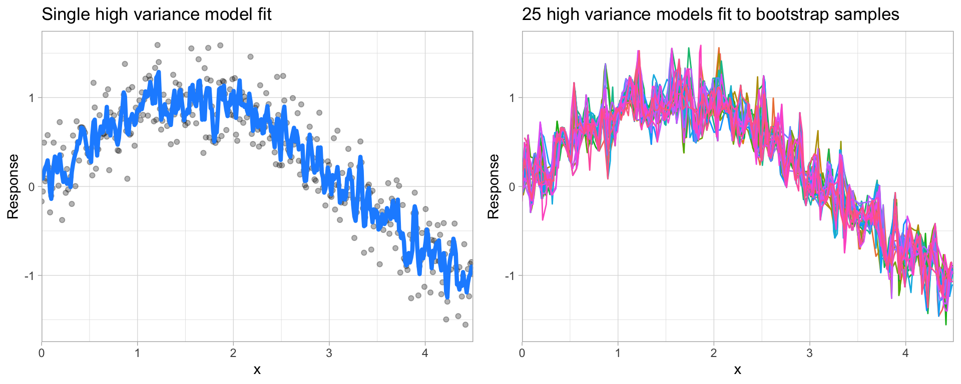
Figure 14.2: A high variance k-nearest neighbor model fit to a single data set captures the underlying non-linear, non-monotonic data structure well but also overfits to individual data points (left). Models fit to 25 bootstrapped replicates of the data are deterred by the noise and generate highly variable predictions (right).

Since high variance models are more prone to overfitting, using resampling procedures are critical to reduce this risk. Moreover, many algorithms that are capable of achieving high generalization performance have lots of hyperparameters that control the level of model complexity (i.e., the tradeoff between bias and variance).

14.3.3 Balancing the tradeoff

We can think of bias and variance as two model attributes competing with one another. If our model is too simple and cannot conform to the relationships in our data then it is underfitting and will not generalize well. If our model is too flexible and overly conforms to the training data then it will also not generalize well. So our objective is to find a model with good balance that does not overfit nor underfit to the training data. This is a model that will generalize well.

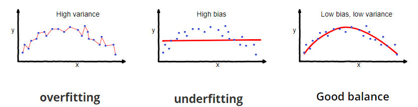
Figure 14.3: Our objective is to find a model with good balance that does not overfit nor underfit to the training data. This is a model that will generalize well.

At its root, dealing with bias and variance is really about dealing with over- and under-fitting. Bias is reduced and variance is increased in relation to model complexity. As more and more hyperparameters are added to a model, the complexity of the model rises and variance becomes our primary concern while bias steadily falls.

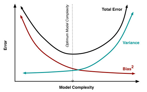
Figure 14.4: As more and more hyperparameters are added to a model, the complexity of the model rises and variance becomes our primary concern while bias steadily falls. The sweet spot for any model is the level of complexity that minimizes bias while keeping variance constrained.

Understanding bias and variance is critical for understanding the behavior of prediction models, but in general what you really care about is overall error, not the specific decomposition. The sweet spot for any model is the level of complexity that minimizes bias while keeping variance constrained. To find this we need an effective and efficient hyperparameter tuning process.

14.4 Hyperparameter tuning

Hyperparameters are the “knobs to twiddle” to control the complexity of machine learning algorithms and, therefore, the bias-variance trade-off. Not all algorithms have hyperparameters; however, as the complexity of our models increase (therefore the ability to capture and conform to more complex relationships in our data) we tend to see an increase in the number of hyperparameters.

The proper setting of these hyperparameters is often dependent on the data and problem at hand and cannot always be estimated by the training data alone. Consequently, we need a method of identifying the optimal setting. For example, in the high variance example in the previous section, we illustrated a high variance k-nearest neighbor model. k-nearest neighbor models have a single hyperparameter (k) that determines the predicted value to be made based on the k nearest observations in the training data to the one being predicted. If k is small (e.g., \(k=3\)), the model will make a prediction for a given observation based on the average of the response values for the 3 observations in the training data most similar to the observation being predicted. This often results in highly variable predicted values because we are basing the prediction (in this case, an average) on a very small subset of the training data. As k gets bigger, we base our predictions on an average of a larger subset of the training data, which naturally reduces the variance in our predicted values (remember this for later, averaging often helps to reduce variance!). The figure below illustrates this point. Smaller k values (e.g., 2, 5, or 10) lead to high variance (but lower bias) and larger values (e.g., 150) lead to high bias (but lower variance). The optimal k value might exist somewhere between 20–50, but how do we know which value of k to use?

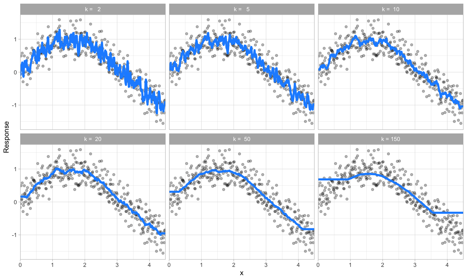
Figure 14.5: k-nearest neighbor model with differing values for k.

One way to perform hyperparameter tuning is to fiddle with hyperparameters manually until you find a great combination of hyperparameter values that result in high predictive accuracy (as measured using k-fold CV, for instance). However, this can be very tedious work depending on the number of hyperparameters. An alternative approach is to perform a grid search. A grid search is an automated approach to searching across many combinations of hyperparameter values.

For the simple example above, a grid search would predefine a candidate set of values for k (e.g., \(k = 1, 2, \dots, j\)) and perform a resampling method (e.g., k-fold CV) to estimate which k value generalizes the best to unseen data. The plots in the below examples illustrate the results from a grid search to assess \(k = 3, 5, \dots, 150\) using repeated 10-fold CV. The error rate displayed represents the average error for each value of k across all the repeated CV folds. On average, \(k=46\) was the optimal hyperparameter value to minimize error (in this case, RMSE which will be discussed shortly) on unseen data.

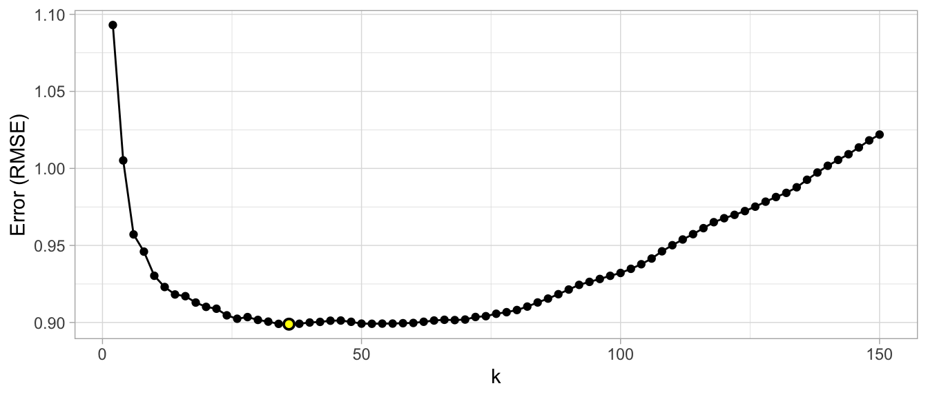
Figure 14.6: Results from a grid search for a k-nearest neighbor model assessing values for k ranging from 3-25. We see high error values due to high model variance when k is small and we also see high errors values due to high model bias when k is large. The optimal model is found at k = 46.

Throughout this course you’ll be exposed to different approaches to performing grid searches. In the above example, we used a full cartesian grid search, which assesses every hyperparameter value manually defined. However, as models get more complex and offer more hyperparameters, this approach can become computationally burdensome and requires you to define the optimal hyperparameter grid settings to explore. Additional approaches we’ll illustrate include random grid searches (Bergstra and Bengio 2012) which explores randomly selected hyperparameter values from a range of possible values, early stopping which allows you to stop a grid search once reduction in the error stops marginally improving, adaptive resampling via futility analysis (Kuhn 2014) which adaptively resamples candidate hyperparameter values based on approximately optimal performance, and more.

14.5 Implementation

Recall our regularized regression model from the last lesson. With that model there are two two main hyperparameters that we need to tune:

• mixture: the type of regularization (ridge, lasso, elastic net) we want to apply and,
• penalty: the strength of the regularization parameter (\(\lambda\)).

Initially, we set mixture = 0 (Ridge model) and the strength of our regularization to penalty = 1000.

# Step 1: create regularized model object
reg_mod <- linear_reg(mixture = 0, penalty = 1000) %>%
   set_engine("glmnet")

# Step 2: create model & preprocessing recipe
model_recipe <- recipe(Sale_Price ~ ., data = ames_train) %>%
   step_normalize(all_numeric_predictors()) %>%
   step_dummy(all_nominal_predictors())

# Step 3. create resampling object
set.seed(123)
kfolds <- vfold_cv(ames_train, v = 5, strata = Sale_Price)

# Step 4: fit model workflow
reg_fit <- workflow() %>%
   add_recipe(model_recipe) %>%
   add_model(reg_mod) %>%
   fit_resamples(kfolds)

# Step 5: assess results
reg_fit %>%
   collect_metrics() %>%
   filter(.metric == 'rmse')
## # A tibble: 1 × 6
##   .metric .estimator   mean     n std_err
##   <chr>   <chr>       <dbl> <int>   <dbl>
## 1 rmse    standard   31373.     5   3012.
## # ℹ 1 more variable: .config <chr>

We then manually iterated through different values of mixture and penalty to try find the optimal setting. Which is less than efficient.

14.5.1 Tuning

Rather than specify set values for mixture and penalty, let’s instead build our model in a way that uses placeholders for values. We can do this using the tune() function:

reg_mod <- linear_reg(mixture = tune(), penalty = tune()) %>%
   set_engine("glmnet")

We can create a regular grid of values to try using some convenience functions for each hyperparameter:

reg_grid <- grid_regular(mixture(), penalty(), levels = 5)

The function grid_regular() is from the dials package. It chooses sensible values to try for each hyperparameter; here, we asked for 5 values each. Since we have two to tune, grid_regular() returns \(5 \times 5 = 25\) different possible tuning combinations to try in a data frame.

reg_grid
## # A tibble: 25 × 2
##    mixture      penalty
##      <dbl>        <dbl>
##  1    0    0.0000000001
##  2    0.25 0.0000000001
##  3    0.5  0.0000000001
##  4    0.75 0.0000000001
##  5    1    0.0000000001
##  6    0    0.0000000316
##  7    0.25 0.0000000316
##  8    0.5  0.0000000316
##  9    0.75 0.0000000316
## 10    1    0.0000000316
## # ℹ 15 more rows

Now that we have our model with hyperparameter value placeholders and a grid of hyperparameter values to assess we can create a workflow object as we’ve done in the past and use tune_grid() to train our 25 models using our k-fold cross validation resamples.

# tune
tuning_results <- workflow() %>%
   add_recipe(model_recipe) %>%
   add_model(reg_mod) %>%
   tune_grid(resamples = kfolds, grid = reg_grid)

# assess results
tuning_results %>%
   collect_metrics() %>%
   filter(.metric == "rmse")
## # A tibble: 25 × 8
##         penalty mixture .metric .estimator
##           <dbl>   <dbl> <chr>   <chr>     
##  1 0.0000000001    0    rmse    standard  
##  2 0.0000000316    0    rmse    standard  
##  3 0.00001         0    rmse    standard  
##  4 0.00316         0    rmse    standard  
##  5 1               0    rmse    standard  
##  6 0.0000000001    0.25 rmse    standard  
##  7 0.0000000316    0.25 rmse    standard  
##  8 0.00001         0.25 rmse    standard  
##  9 0.00316         0.25 rmse    standard  
## 10 1               0.25 rmse    standard  
## # ℹ 15 more rows
## # ℹ 4 more variables: mean <dbl>, n <int>,
## #   std_err <dbl>, .config <chr>

We can assess our best models with show_best(), which by default will show the top 5 performing models based on the desired metric. In this case we see that our top 5 models use the Ridge regularization (mixture = 0) and across all the penalties we get the same cross-validation RMSE (31,373).

tuning_results %>%
   show_best(metric = "rmse")
## # A tibble: 5 × 8
##    penalty mixture .metric .estimator   mean
##      <dbl>   <dbl> <chr>   <chr>       <dbl>
## 1 1   e-10       0 rmse    standard   31373.
## 2 3.16e- 8       0 rmse    standard   31373.
## 3 1   e- 5       0 rmse    standard   31373.
## 4 3.16e- 3       0 rmse    standard   31373.
## 5 1   e+ 0       0 rmse    standard   31373.
## # ℹ 3 more variables: n <int>,
## #   std_err <dbl>, .config <chr>

We can also use the select_best() function to pull out the single set of hyperparameter values for our best regularization model:

tuning_results %>%
   select_best("rmse")
## # A tibble: 1 × 3
##        penalty mixture .config              
##          <dbl>   <dbl> <chr>                
## 1 0.0000000001       0 Preprocessor1_Model01

14.5.2 More tuning

Based on the above results, we may wish to do another iteration and adjust the hyperparameter values to assess. Since all our best models were Ridge models we may want to set our model to use a Ridge penalty but then just tune the strength of the penalty.

Here, we create another hyperparameter grid but we specify the range we want to search through. Note that penalty automatically applies a log transformation so by saying range = c(0, 5) I am actually saying to search between 1 - 100,000.

reg_mod <- linear_reg(mixture = 0, penalty = tune()) %>%
   set_engine("glmnet")

reg_grid <- grid_regular(penalty(range = c(0, 5)), levels = 10)

Now we can search again and we see that by using slightly higher penalty values we improve our performance.

tuning_results <- workflow() %>%
   add_recipe(model_recipe) %>%
   add_model(reg_mod) %>%
   tune_grid(resamples = kfolds, grid = reg_grid)

tuning_results %>%
   show_best(metric = "rmse")
## # A tibble: 5 × 7
##    penalty .metric .estimator   mean     n
##      <dbl> <chr>   <chr>       <dbl> <int>
## 1 27826.   rmse    standard   30633.     5
## 2  7743.   rmse    standard   31160.     5
## 3     1    rmse    standard   31373.     5
## 4     3.59 rmse    standard   31373.     5
## 5    12.9  rmse    standard   31373.     5
## # ℹ 2 more variables: std_err <dbl>,
## #   .config <chr>

14.5.3 Finalizing our model

We can update (or “finalize”) our workflow object with the values from select_best(). This now creates a final model workflow with the optimal hyperparameter values.

best_hyperparameters <- select_best(tuning_results, metric = "rmse")

final_wf <- workflow() %>%
   add_recipe(model_recipe) %>%
   add_model(reg_mod) %>% 
   finalize_workflow(best_hyperparameters)

final_wf
## ══ Workflow ════════════════════════════════
## Preprocessor: Recipe
## Model: linear_reg()
## 
## ── Preprocessor ────────────────────────────
## 2 Recipe Steps
## 
## • step_normalize()
## • step_dummy()
## 
## ── Model ───────────────────────────────────
## Linear Regression Model Specification (regression)
## 
## Main Arguments:
##   penalty = 27825.5940220713
##   mixture = 0
## 
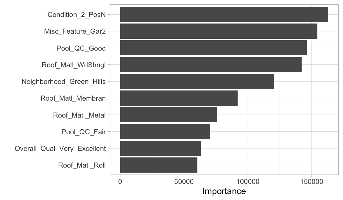
## Computational engine: glmnet

We can then use this final workflow to do further assessments. For example, if we want to train this workflow on the entire data set and look at which predictors are most influential we can:

final_wf %>%
   fit(data = ames_train) %>% 
   extract_fit_parsnip() %>% 
   vip()

14.6 Exercises

Using the same kernlab::spam data we saw in the section 12.10…

1. Split the data into 70-30 training-test sets.
2. Apply a regularized classification model (type is our response variable) but use the tune() and grid_regular() approach we saw in this lesson to automatically tune the mixture and penalty hyperparameters. Use a 5-fold cross-validation procedure.
3. Which hyperparameter values maximize the AUC (roc_auc) metric?
4. Retrain a final model with these optimal hyperparameters and identify the top 10 most influential predictors.

References

Bergstra, James, and Yoshua Bengio. 2012. “Random Search for Hyper-Parameter Optimization.” Journal of Machine Learning Research 13 (Feb): 281–305.

Kuhn, Max. 2014. “Futility Analysis in the Cross-Validation of Machine Learning Models.” arXiv Preprint arXiv:1405.6974.