19 Lesson 6c: Random Forests
Random forests are a modification of bagged decision trees that build a large collection of de-correlated trees to further improve predictive performance. They have become a very popular “out-of-the-box” or “off-the-shelf” learning algorithm that enjoys good predictive performance with relatively little hyperparameter tuning. Many modern implementations of random forests exist; however, Leo Breiman’s algorithm (Breiman 2001) has largely become the authoritative procedure. This module will cover the fundamentals of random forests.
19.1 Learning objectives
By the end of this module you will know:
- How to implement a random forest model along with the hyperparameters that are commonly toggled in these algorithms.
- Multiple strategies for performing a grid search.
- How to identify influential features and their effects on the response variable.
19.2 Prerequisites
19.3 Extending bagging
Random forests are built using the same fundamental principles as decision trees and bagging. Bagging trees introduces a random component into the tree building process by building many trees on bootstrapped copies of the training data. Bagging then aggregates the predictions across all the trees; this aggregation reduces the variance of the overall procedure and results in improved predictive performance. However, as we saw in the last module, simply bagging trees results in tree correlation that limits the effect of variance reduction.
Random forests help to reduce tree correlation by injecting more randomness into the tree-growing process.9 More specifically, while growing a decision tree during the bagging process, random forests perform split-variable randomization where each time a split is to be performed, the search for the split variable is limited to a random subset of \(m_{try}\) of the original \(p\) features. Typical default values are \(m_{try} = \frac{p}{3}\) (regression) and \(m_{try} = \sqrt{p}\) (classification) but this should be considered a tuning parameter.
The basic algorithm for a regression or classification random forest can be generalized as follows:
1.  Given a training data set
2.  Select number of trees to build (n_trees)
3.  for i = 1 to n_trees do
4.  |  Generate a bootstrap sample of the original data
5.  |  Grow a regression/classification tree to the bootstrapped data
6.  |  for each split do
7.  |  | Select m_try variables at random from all p variables
8.  |  | Pick the best variable/split-point among the m_try
9.  |  | Split the node into two child nodes
10. |  end
11. | Use typical tree model stopping criteria to determine when a
    | tree is complete (but do not prune)
12. end
13. Output ensemble of trees
When \(m_{try} = p\), the algorithm is equivalent to bagging decision trees.
Since the algorithm randomly selects a bootstrap sample to train on and a random sample of features to use at each split, a more diverse set of trees is produced which tends to lessen tree correlation beyond bagged trees and often dramatically increase predictive power.
19.4 Out-of-the-box performance
Random forests have become popular because they tend to provide very good out-of-the-box performance. Although they have several hyperparameters that can be tuned, the default values tend to produce good results. Moreover, Probst, Bischl, and Boulesteix (2018) illustrated that among the more popular machine learning algorithms, random forests have the least variability in their prediction accuracy when tuning.
For example, if we train a random forest model with all hyperparameters set to their default values, we get RMSEs comparable to some of the best model’s we’ve run thus far (without any tuning).
In R we will want to use the ranger package as our random forest engine. Similar to other examples we need to set the mode of machine learning model to either a regression or classification modeling objective.
# create model recipe with all features
model_recipe <- recipe(
    Sale_Price ~ .,
    data = ames_train
  )

# create random forest model object
rf_mod <- rand_forest(mode = "regression") %>%
  set_engine("ranger")

# create resampling procedure
set.seed(13)
kfold <- vfold_cv(ames_train, v = 5)

# train model
results <- fit_resamples(rf_mod, model_recipe, kfold)

# model results
collect_metrics(results)
## # A tibble: 2 × 6
##   .metric .estimator      mean     n    std_err .config
##   <chr>   <chr>          <dbl> <int>      <dbl> <chr>
## 1 rmse    standard   26981.        5 1119.      Preprocessor1_Model1
## 2 rsq standard 0.895 5 0.00862 Preprocessor1_Model119.5 Hyperparameters
Although random forests perform well out-of-the-box, there are several tunable hyperparameters that we should consider when training a model. Although we briefly discuss the main hyperparameters, Probst, Wright, and Boulesteix (2019) provide a much more thorough discussion. The main hyperparameters to consider include:
- The number of trees in the forest
- The number of features to consider at any given split: \(m_{try}\)
- The complexity (depth) of each tree
19.5.1 Number of trees
The first consideration is the number of trees within your random forest. Although not technically a hyperparameter, the number of trees needs to be sufficiently large to stabilize the error rate. A good rule of thumb is to start with 10 times the number of features as illustrated below); however, as you adjust other hyperparameters such as \(m_{try}\) and node size, more or fewer trees may be required. More trees provide more robust and stable error estimates and variable importance measures; however, the impact on computation time increases linearly with the number of trees.
A good rule of thumb is to start with the number of predictor variables (\(p\)) times 10 (\(p \times 10\)) trees and adjust as necessary.
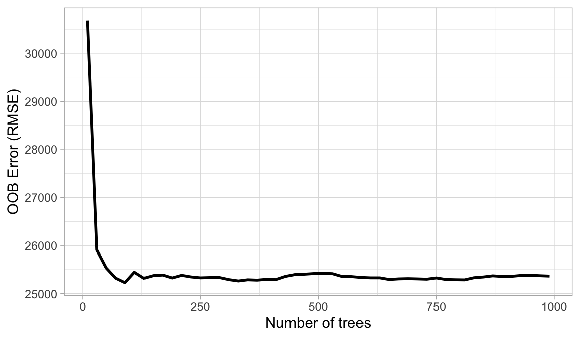
Figure 19.1: The Ames data has 80 features and starting with 10 times the number of features typically ensures the error estimate converges.
19.5.2 \(m_{try}\)
The hyperparameter that controls the split-variable randomization feature of random forests is often referred to as \(m_{try}\) and it helps to balance low tree correlation with reasonable predictive strength. With regression problems the default value is often \(m_{try} = \frac{p}{3}\) and for classification \(m_{try} = \sqrt{p}\). However, when there are fewer relevant predictors (e.g., noisy data) a higher value of \(m_{try}\) tends to perform better because it makes it more likely to select those features with the strongest signal. When there are many relevant predictors, a lower \(m_{try}\) might perform better.
Start with five evenly spaced values of \(m_{try}\) across the range 2–\(p\) centered at the recommended default as illustrated below. For the Ames data, an mtry value slightly lower (21) than the default (26) improves performance.
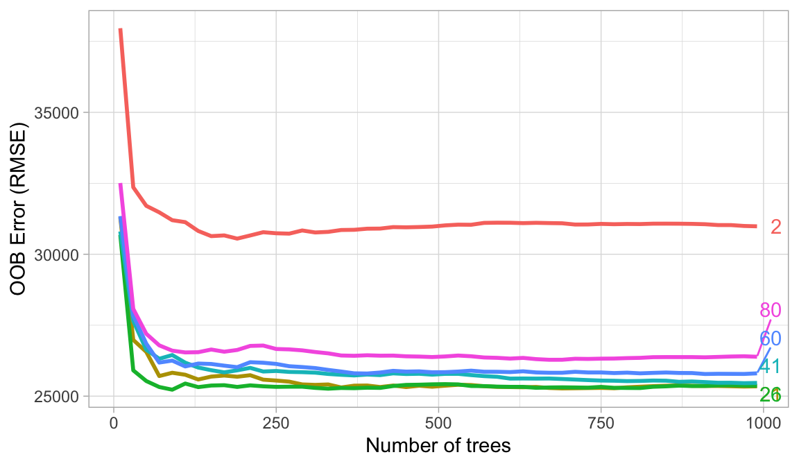
Figure 19.2: For the Ames data, an mtry value in the low to mid 20s improves performance.
19.5.3 Tree complexity
Random forests are built on individual decision trees; consequently, most random forest implementations have one or more hyperparameters that allow us to control the depth and complexity of the individual trees. This will often include hyperparameters such as node size, max depth, max number of terminal nodes, or the required node size to allow additional splits. Node size is probably the most common hyperparameter to control tree complexity and most implementations use the default values of one for classification and five for regression as these values tend to produce good results (Dı́az-Uriarte and De Andres 2006; Goldstein, Polley, and Briggs 2011). However, Segal (2004) showed that if your data has many noisy predictors and higher \(m_{try}\) values are performing best, then performance may improve by increasing node size (i.e., decreasing tree depth and complexity). Moreover, if computation time is a concern then you can often decrease run time substantially by increasing the node size and have only marginal impacts to your error estimate as illustrated below.
When adjusting node size start with three values between 1–10 and adjust depending on impact to accuracy and run time. Increasing node size to reduce tree complexity will often have a larger impact on computation speed (right) than on your error estimate.
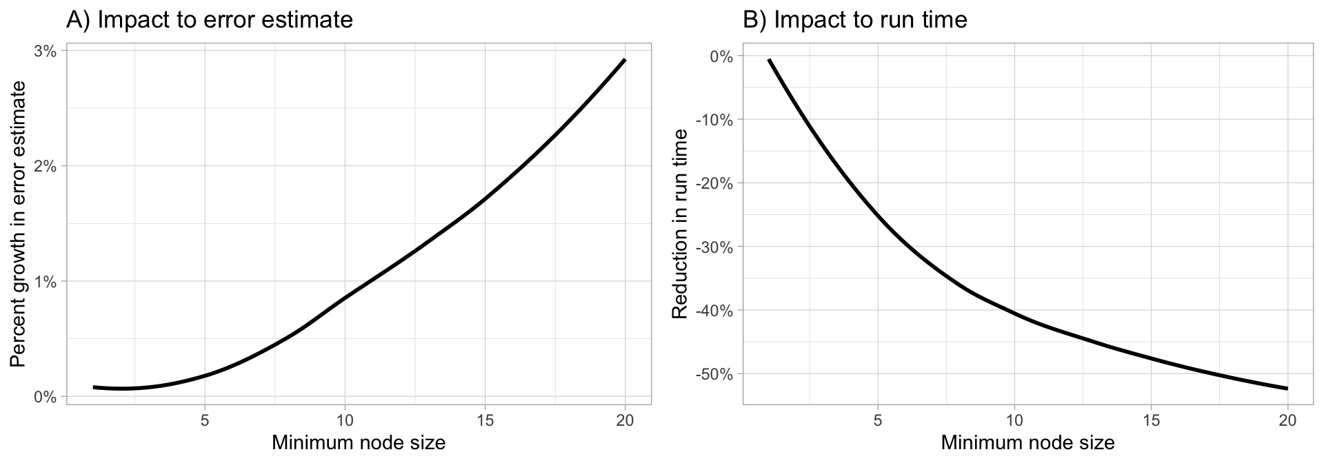
Figure 19.3: Increasing node size to reduce tree complexity will often have a larger impact on computation speed (right) than on your error estimate.
19.5.4 Others
There are many other hyperparameters within random forest models; however, the above mentioned ones are the most common and, often, most influential in the performance of our model. For more discussion around random forest hyperparameters see Probst, Wright, and Boulesteix (2019).
19.6 Tuning
The following performs a grid search over the mtry (number of features to randomly use for a given tree) and min_n (controls tree depth) hyperparameters. Notice how we don’t actually tune the trees parameter. Rather, setting this to a value greater than the number of features \(\times\) 10 is sufficient. Since we have 80 features we set it to at least, if not greater than \(80 \times 10 = 800\).
The following grid search results in a search of 25 different hyperparameter combinations, which results in a grid search time of about 14 minutes!
Also, note the importance = “impurity” code we added to
set_engine(). We’ll discuss why we add this shortly.
# create random forest model object with tuning option
rf_mod <- rand_forest(
  mode = "regression",
  trees = 1000,
  mtry = tune(),
  min_n = tune()
  ) %>%
  set_engine("ranger", importance = "permutation")

# create the hyperparameter grid
hyper_grid <- grid_regular(
   mtry(range = c(2, 80)),
   min_n(range = c(1, 20)),
   levels = 5
   )

# train our model across the hyper parameter grid
set.seed(123)
results <- tune_grid(rf_mod, model_recipe, resamples = kfold, grid = hyper_grid)

# model results
show_best(results, metric = "rmse")
## # A tibble: 5 × 8
##    mtry min_n .metric .estimator   mean     n std_err .config
##   <int> <int> <chr>   <chr>       <dbl> <int>   <dbl> <chr>
## 1    41     1 rmse    standard   25988.     5   1021. Preprocessor1_Mo…
## 2    60     1 rmse    standard   26151.     5   1106. Preprocessor1_Mo…
## 3    21     5 rmse    standard   26167.     5   1109. Preprocessor1_Mo…
## 4    21     1 rmse    standard   26207.     5   1113. Preprocessor1_Mo…
## 5    41     5 rmse    standard   26223.     5   1052. Preprocessor1_Mo…
19.6.1 Knowledge check
Using the boston.csv dataset:
Apply a random forest model where cmedv is the response
variable and use all possible predictor variables. Use a 5-fold cross
validation procedure and tune mtry, min_n, and
trees. Assess 3 levels of each hyperparameter ranging
from:
-
trees: use a range from 50-500 -
mtry: use a range from 2-15 -
min_n: use a range 1-10
Which combination of hyperparameters perform best. What is the lowest cross-validated RMSE and how does this compare to previous models on the boston data?
19.7 Feature interpretation
Computing feature importance and feature effects for random forests follow the same procedure as discussed in the bagging module. For each tree in our random forest, we compute the sum of the reduction of the loss function across all splits for a given predictor variable. We then aggregate this measure across all trees for each feature. The features with the largest average decrease in SSE (for regression) are considered most important.
This is called the “impurity” method for computing feature
importance. And to get this measure for our random forests we need to
add importance = “impurity” to set_engine() as
we did in the last section.
# get optimal hyperparameters
best_hyperparameters <- select_best(results, metric = "rmse")

# create final workflow object
final_rf_wf <- workflow() %>%
   add_recipe(model_recipe) %>%
   add_model(rf_mod) %>%
   finalize_workflow(best_hyperparameters)

# fit final workflow object
final_fit <- final_rf_wf %>%
   fit(data = ames_train)

# plot feature importance
final_fit %>%
   extract_fit_parsnip() %>%
   vip(num_features = 20)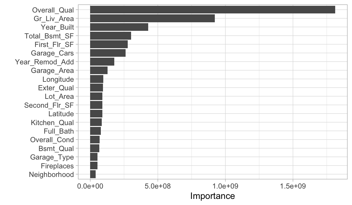
We can then plot the partial dependence of the most influential feature to see how it influences the predicted values. We see that as overall quality increase we see a significant increase in the predicted sale price.
# prediction function
pdp_pred_fun <- function(object, newdata) {
   predict(object, newdata, type = "numeric")$.pred
}

# use the pdp package to extract partial dependence predictions
# and then plot
final_fit %>%
   pdp::partial(
     pred.var = "Overall_Qual",
     pred.fun = pdp_pred_fun,
     grid.resolution = 10,
     train = ames_train
   ) %>%
  ggplot(aes(Overall_Qual, yhat)) +
    geom_boxplot() +
    scale_y_continuous(labels = scales::dollar)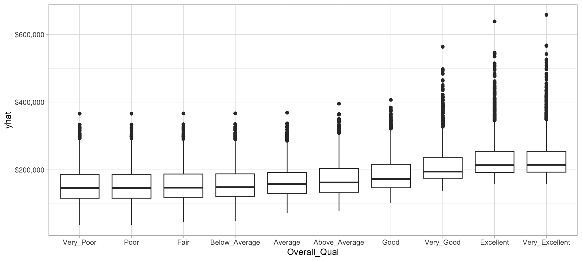
Now let’s plot the PDP for the Gr_Liv_Area and see how that variable relates to the predicted sale price.
# prediction function
pdp_pred_fun <- function(object, newdata) {
   mean(predict(object, newdata, type = "numeric")$.pred)
}

# use the pdp package to extract partial dependence predictions
# and then plot
final_fit %>%
   pdp::partial(
     pred.var = "Gr_Liv_Area",
     pred.fun = pdp_pred_fun,
     grid.resolution = 10,
     train = ames_train
   ) %>%
   autoplot() +
   scale_y_continuous(labels = scales::dollar)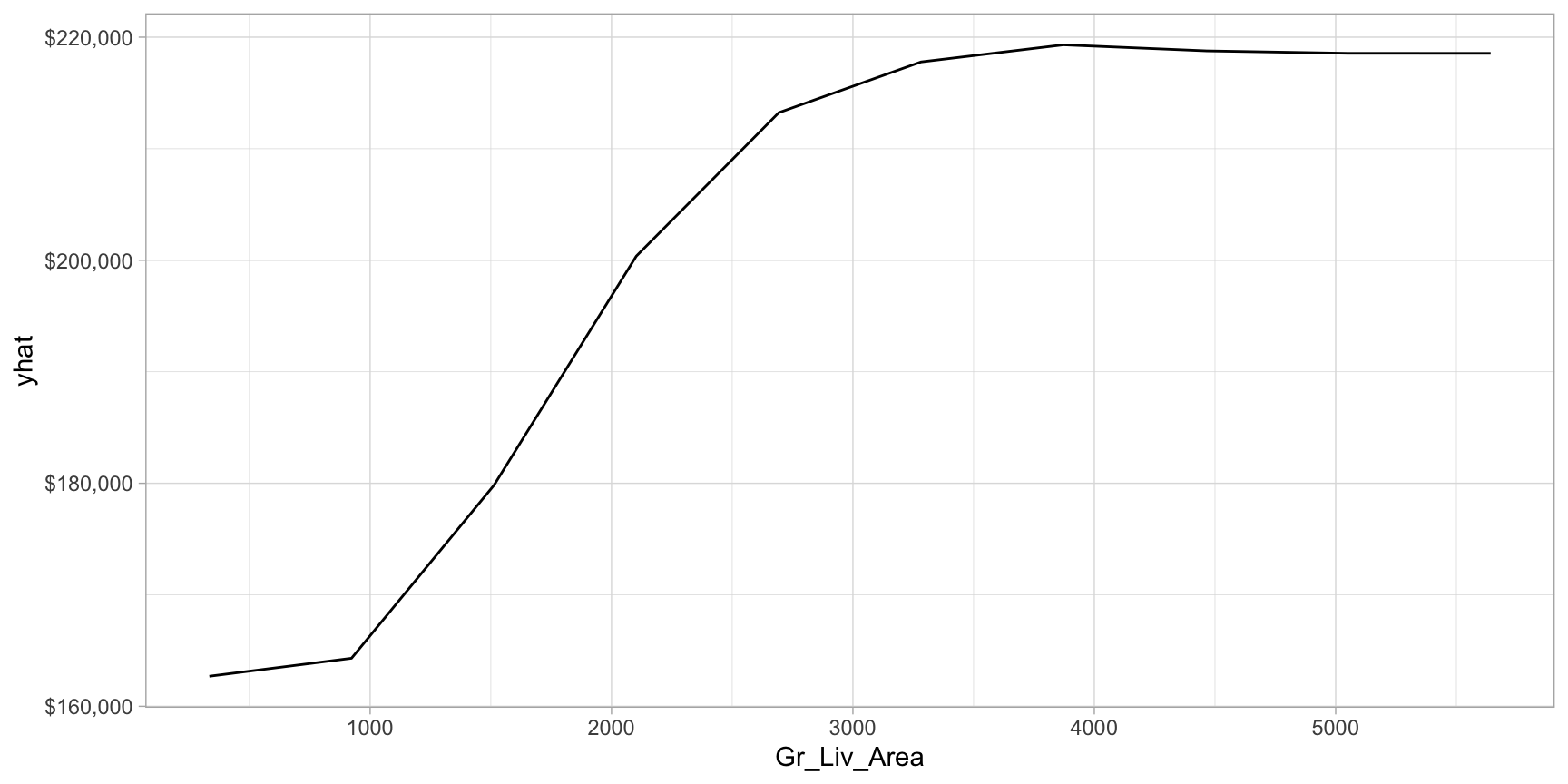
19.8 Final thoughts
Random forests provide a very powerful out-of-the-box algorithm that often has great predictive accuracy. They come with all the benefits of decision trees (with the exception of surrogate splits) and bagging but greatly reduce instability and between-tree correlation. And due to the added split variable selection attribute, random forests are also faster than bagging as they have a smaller feature search space at each tree split. However, random forests will still suffer from slow computational speed as your data sets get larger but, similar to bagging, the algorithm is built upon independent steps, and most modern implementations allow for parallelization to improve training time.
19.9 Exercises
Using the same kernlab::spam data we saw in the section
12.10…
- Split the data into 70-30 training-test sets.
-
Apply a default random forest model modeling the
typeresponse variable as a function of all available features. -
Now tune the
trees,mtry, andmin_nhyperparameters to find the best performing combination of hyperparameters. - How does the model performance compare to the decision tree model and bagged decision tree model applied in the previous two lesson exercises?
- Which 10 features are considered most influential? Are these the same features that have been influential in previous models?
- Create partial dependence plots for the top two most influential features. Explain the relationship between the feature and the predicted values.