Lesson 0: Configuring your computer#
In this lesson, you will set up a Python computing environment for scientific computing (aka data science). There are two main ways people set up Python for scientific computing on their own machine.
By downloading and installing package by package with tools like apt-get, pip, etc.
By downloading and installing a Python distribution that contains binaries of many of the scientific packages needed. One widely used distribution is from Anaconda.
In this class, we will use Anaconda, with its associated package manager, conda. It has become the de facto package manager/distribution for scientific use.
Learning objectives#
By the end of this lesson you will:
Have an updated version of Python installed on your computer.
Be able to launch JupyterLab.
Have all required packages for this course installed.
Why install on my own machine?#
I toyed with using Google Colab for this class, and I may in fact encourage you to use it when you are working on exercises. This offers many advantages.
You get a dedicated powerful machine that is part of Google’s cloud resources for your computing.
Most of what you need is pre-installed.
You can easily share the notebook with collaborators in near-real time.
It is free!
There are many more advanced features that are not covered in the class, such as easy GPU computing.
I chose not to do this for several reasons, the first being the most important.
It is important that you learn how to set up your own machine, including using the command line.
Unless you have a pro account (not free), your Colab instance will shut down after a period of latency.
It is not as easy to integrate into your own software development pipeline.
Along those same lines, it is not as easy to install custom software, or software that you write, using Colab as it is on your own machine.
You may also want to use other cloud computing resources like AWS, Microsoft Azure, or Caltech’s HPC. We are not using those because we do not need more computing power than is available on a standard laptop. Furthermore, setting up your own machine will help prepare you for setting up instances on those services.
Before we get rolling with the Anaconda distribution on your own machine, we have some considerations and installations to get out of the way first.
macOS users: Install XCode#
If you are using macOS, you should install XCode, if you haven’t already. You can install it through the App Store.
Warning
It’s a large piece of software, taking up about 5GB on your hard drive, so make sure you have enough space. Also, this will take a long time to install.
After installing it, you need to open the program. Be sure to do that, for example by clicking on the XCode icon in your Applications folder. Upon opening XCode, it may perform more installations. You can let it go ahead and do this, and then close XCode.
Windows users: Install Git and Chrome or Firefox#
We will be using JupyterLab in this class. It is browser-based, and Chrome, Firefox, and Safari are supported. Microsoft Edge is not. Therefore, if you are a Windows user, you need to be sure you have either Chrome of Firefox installed.
Git is installed on Macs with XCode. For Windows users, you need to install Git. You can do this by following the instructions here.
Uninstalling Anaconda#
If you have previously installed Anaconda with a version of Python other than 3.8, you need to uninstall it, removing it completely from your computer. You can find instructions on how to do that from the official uninstallation documentation.
Downloading and installing Anaconda#
Downloading and installing Anaconda is simple.
Go to the Anaconda homepage and download the graphical installer.
Install Anaconda with Python 3.8 or higher.
You may be prompted for your email address, which you should provide. You may want to use your university email address because educational users can get some of the non-free goodies in Anaconda.
Follow the on-screen instructions for installation. While doing so, be sure that Anaconda is installed in your home directory, not in root.
That’s it! After you do that, you will have a functioning Python distribution.
Installing node.js#
node.js is a platform that enables you to run JavaScript outside of the browser. We will not use it directly, but it needs to be installed for some of the more sophisticated JupyterLab functionality. Install node.js by following the instructions here.
Launching JupyterLab and a terminal#
You can launch JupyterLab via the Anaconda Navigator or via your operating system’s terminal program (Terminal on macOS and PowerShell on Windows). If you wish to launch using the latter, skip to the next section.
If you’re using macOS, Anaconda Navigator will be available in your Applications menu. If you are using Windows, you can launch Anaconda Navigator from the Start menu.
We will be using JupyterLab throughout the class (more on that in the next lesson). You should see an option to launch JupyterLab from within Anaconda Navigator.
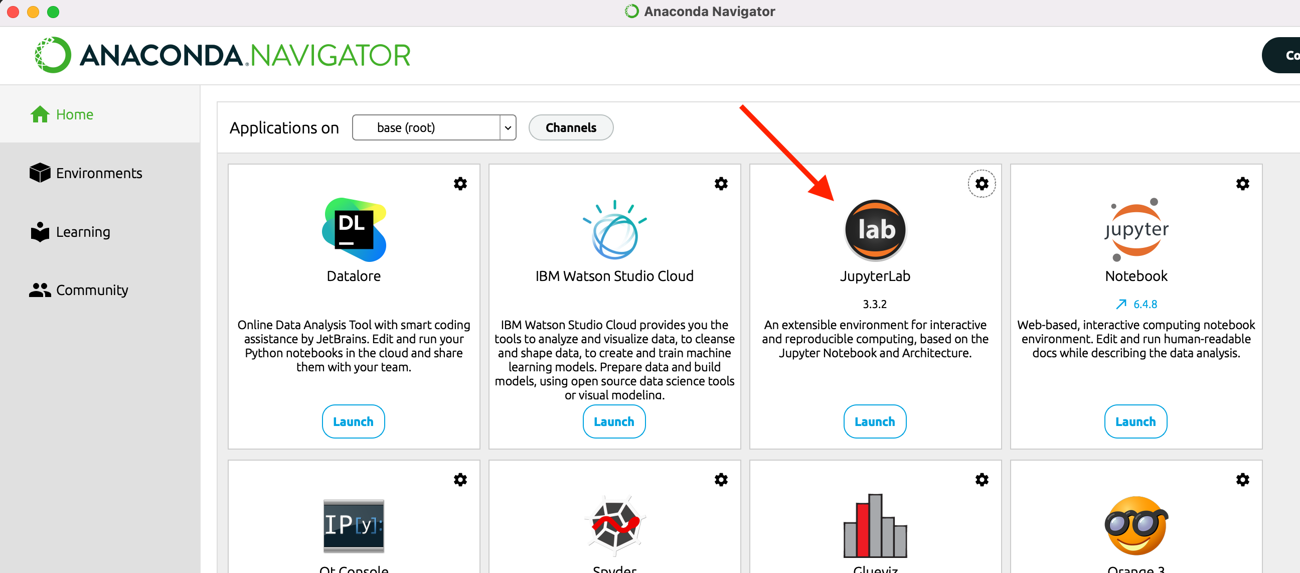
Fig. 1 The Anaconda Navigator.#
When you do that, a new browser window or tab will open with JupyterLab running. Within the JupyterLab window, you will have the option to launch a notebook, a console, a terminal, text file, Python file, etc. We will use many of these during the class.
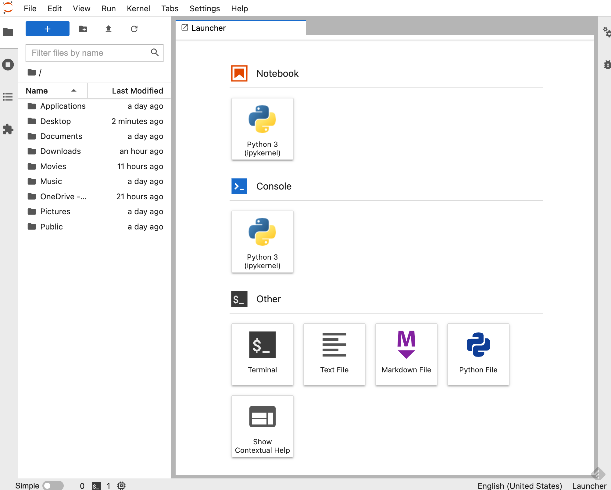
Fig. 2 Jupyter Lab landing page.#
For the updating and installation of necessary packages, click on Terminal to launch a terminal. You will get a terminal window (probably black) with a bash prompt. We refer to this text interface in the terminal as the command line.
Launching JupyterLab from the command line#
While launching JupyterLab from the Anaconda Navigator is fine, I generally prefer to launch it from the command line on my own machine. If you are on a Mac, open the Terminal program. You can do this hitting Command + space bar and searching for “terminal.” Using Windows, you should launch PowerShell. You can do this by hitting Windows + R and typing powershell in the text box.
Once you have a terminal or PowerShell window open, you will have a prompt. At the prompt, type
jupyter lab
and you will have an instance of JupyterLab running in your browser. If you want to specify the browser, you can, for example, type
jupyter lab --browser=firefox
on the command line.
It is up to you if you want to launch JupyterLab from the Anaconda Navigator or command line.
Note
On many platforms, Jupyter will automatically open up in your default web browser (unless you start it with --no-browser). Otherwise, you can navigate to the HTTP address printed when you started the notebook, here http://localhost:8888/.
Tip
If you are using PowerShell and get an error along the lines of jupyter : The term 'jupyter' is not recognized... when trying to launch jupyter lab, then try opening PowerShell from Anaconda Navigator instead of the main Windows PowerShell app.
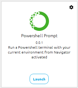
Fig. 3 Launch PowerShell via Anaconda.#
The conda package manager#
conda is a package manager for keeping all of your packages up-to-date. It has plenty of functionality beyond our basic usage in class, which you can learn more about by reading the docs. We will primarily be using conda to install and update packages.
conda works from the command line. Now that you know how to get a command line prompt, you can start using conda. The first thing we’ll do is update conda itself. Enter the following on the command line.
conda update conda
You can press y to continue. You should do this once more, again entering
conda update conda
on the commmand line.
Next, we will update the packages that came with the Anaconda distribution. To do this, enter the following on the command line:
conda update --all
If anything is out of date, you will be prompted to perform the updates, and press y to continue. (If everything is up to date, you will just see a list of all the installed packages.) They may even be some downgrades. This happens when there are package conflicts where one package requires an earlier version of another. conda is very smart and figures all of this out for you, so you can almost always say “yes” (or “y”) to conda when it prompts you.
Note
If you are new to conda do not worry, we will spend a lesson focusing on conda and more advanced ways to use it. For now, we just want to use it to update all the packages you’ll use throughout this class.
Installations#
There are several additional installations of Python packages you need to do for this class. Many of these packages are available through conda. First, we need to install jupyter_bokeh, which allows Bokeh plots to be displayed withing Jupyter notebooks. Do the following on the command line.
conda install -c bokeh jupyter_bokeh
Now, we can proceed with the rest of our installations.
conda install matplotlib numpy pandas scipy seaborn scikit-learn sqlalchemy
There are a few other packages from pip we will need for the class, so we can go ahead and install those now.
pip install blackcellmagic completejourney_py iqplot jupyterlab-spellchecker watermark
You should close your JupyterLab session and terminate Anaconda Navigator after you have completed the build. Relaunch Anaconda Navigator and launch a fresh JupyterLab instance.
Note
Again do not worry if you are not familiar with what packages are or what is happening when you run the code above. We will discuss this further in a future model.
Checking your distribution#
We’ll now run a quick test to make sure things are working properly. We will make a quick plot that requires some of the scientific libraries we will use in this class.
Use the JupyterLab launcher (you can get a new launcher by clicking on the + icon on the left pane of your JupyterLab window) to launch a notebook. In the first cell (the box next to the [ ]: prompt), paste the code below. To run the code, press Shift+Enter while the cursor is active inside the cell. You should see a plot that looks like the one below. If you do, you have a functioning Python environment for scientific computing!
import numpy as np
import bokeh.plotting
import bokeh.io

bokeh.io.output_notebook()

# Generate plotting values
t = np.linspace(0, 2*np.pi, 200)
x = 16 * np.sin(t)**3
y = 13 * np.cos(t) - 5 * np.cos(2*t) - 2 * np.cos(3*t) - np.cos(4*t)

p = bokeh.plotting.figure(height=250, width=275)
p.line(x, y, color='red', line_width=3)
text = bokeh.models.Label(x=0, y=0, text='BANA 6043', text_align='center')
p.add_layout(text)

bokeh.io.show(p)
Computing environment#
%load_ext watermark
%watermark -v -p numpy,bokeh,jupyterlab
Python implementation: CPython
Python version       : 3.12.4
IPython version      : 8.26.0

numpy     : 2.0.0
bokeh     : 3.4.2
jupyterlab: 4.2.3