Lession 4a: Tidy data

Lession 4a: Tidy data#

Tidy data is about “linking the structure of a dataset with its semantics (its meaning)”. It is defined by:

Each variable forms a column
Each observation forms a row
Each type of observational unit forms a table

Often you’ll need to reshape a dataframe to make it tidy (or for some other purpose).

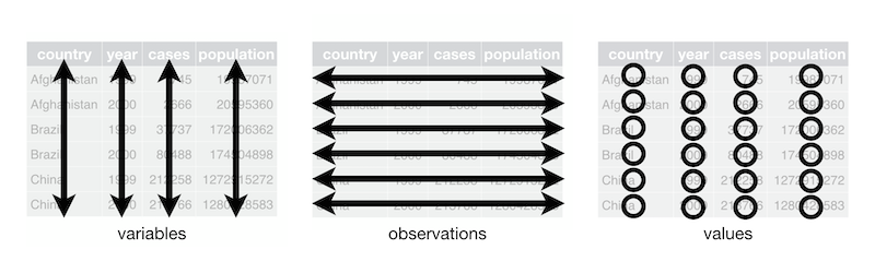
Source: R4DS

Once a DataFrame is tidy, it becomes much easier to compute summary statistics, join with other datasets, visualize, apply machine learning models, etc. In this lesson we will focus on ways to reshape DataFrames so that they meet the tidy guidelines.

Video 🎥:

Learning objectives#

By the end of this lesson you will be able to:

Reshape data from wide to long
Reshape data from long to wide

Tools for reshaping#

Pandas provides multiple methods that help to reshape DataFrames:

.melt(): make wide data long.
.pivot(): make long data width.
.pivot_table(): same as .pivot() but can handle multiple indexes.

Source: Garrick Aden-Buie

The following will illustrate each of these for their unique purpose.

Melting wide data#

The below data shows how many homes were sold within each neighborhood across each year. Is this considered ‘tidy data’? No because we have a variable (year sold) that is represented as the columns and another variable (number of homes sold) filled in as the element values.

If you wanted to answer questions like: “Does the number of homes sold vary depending on year?” then the below data is not in the appropriate form to answer this question.

import pandas as pd

ames_wide = pd.read_csv('../data/ames_wide.csv')
ames_wide.head()

	neighborhood	2006	2007	2008	2009	2010
0	Blmngtn	11.0	4.0	5.0	6.0	2.0
1	Blueste	NaN	2.0	2.0	4.0	2.0
2	BrDale	9.0	5.0	7.0	6.0	3.0
3	BrkSide	19.0	24.0	31.0	23.0	11.0
4	ClearCr	10.0	9.0	11.0	6.0	8.0

In this example we would consider this data “wide” and our objective is to convert it into a DataFrame with three variables:

neighborhood
year
homes_sold

To do so we’ll use the .melt() method. .melt() arguments include:

id_vars: Identifier column
var_name: Name to give the new variable represented by the old column headers
value_name: Name to give the new variable represented by the old element values

ames_melt = ames_wide.melt(id_vars='neighborhood', var_name='year', value_name='homes_sold')
ames_melt

	neighborhood	year	homes_sold
0	Blmngtn	2006	11.0
1	Blueste	2006	NaN
2	BrDale	2006	9.0
3	BrkSide	2006	19.0
4	ClearCr	2006	10.0
...	...	...	...
135	SawyerW	2010	18.0
136	Somerst	2010	21.0
137	StoneBr	2010	6.0
138	Timber	2010	8.0
139	Veenker	2010	NaN

140 rows × 3 columns

The value_vars argument allows us to select which specific variables we want to “melt” (if you don’t specify value_vars, all non-identifier columns will be used). For example, below I’m omitting the 2006 column:

ames_wide.melt(
    id_vars='neighborhood',
    value_vars=['2007', '2008', '2009', '2010'],
    var_name='year',
    value_name='homes_sold'
    )

	neighborhood	year	homes_sold
0	Blmngtn	2007	4.0
1	Blueste	2007	2.0
2	BrDale	2007	5.0
3	BrkSide	2007	24.0
4	ClearCr	2007	9.0
...	...	...	...
107	SawyerW	2010	18.0
108	Somerst	2010	21.0
109	StoneBr	2010	6.0
110	Timber	2010	8.0
111	Veenker	2010	NaN

112 rows × 3 columns

Knowledge check#

Questions:

Given the following DataFrame, reshape the DataFrame from the current “wide” format to a “longer” format made up of the following variables:

Name: will contain the same values in the current Name column,
Year: will contain the year values which are currently column names, and
Courses: will contain the values that are currently listed under each year variable.

df = pd.DataFrame({"Name": ["Tom", "Mike", "Tiffany", "Varada", "Joel"],
                   "2018": [1, 3, 4, 5, 3],
                   "2019": [2, 4, 3, 2, 1],
                   "2020": [5, 2, 4, 4, 3]})
df

	Name	2018	2019	2020
0	Tom	1	2	5
1	Mike	3	4	2
2	Tiffany	4	3	4
3	Varada	5	2	4
4	Joel	3	1	3

Video 🎥:

Pivoting long data#

Sometimes, you want to make long data wide, which we can do with .pivot(). When using .pivot() we need to specify the index to pivot on, and the columns that will be used to make the new columns of the wider dataframe. Let’s convert our ames_melt DataFrame back to the wide format:

ames_pivot = ames_melt.pivot(index='neighborhood', columns='year', values='homes_sold')
ames_pivot

year	2006	2007	2008	2009	2010
neighborhood
Blmngtn	11.0	4.0	5.0	6.0	2.0
Blueste	NaN	2.0	2.0	4.0	2.0
BrDale	9.0	5.0	7.0	6.0	3.0
BrkSide	19.0	24.0	31.0	23.0	11.0
ClearCr	10.0	9.0	11.0	6.0	8.0
CollgCr	60.0	65.0	58.0	63.0	21.0
Crawfor	20.0	34.0	21.0	21.0	7.0
Edwards	43.0	41.0	45.0	42.0	23.0
Gilbert	38.0	45.0	26.0	41.0	15.0
Greens	4.0	1.0	NaN	1.0	2.0
GrnHill	1.0	1.0	NaN	NaN	NaN
IDOTRR	20.0	25.0	26.0	13.0	9.0
Landmrk	1.0	NaN	NaN	NaN	NaN
MeadowV	10.0	8.0	7.0	5.0	7.0
Mitchel	23.0	28.0	22.0	24.0	17.0
NAmes	99.0	105.0	86.0	95.0	58.0
NPkVill	3.0	3.0	3.0	10.0	4.0
NWAmes	25.0	30.0	30.0	35.0	11.0
NoRidge	17.0	17.0	14.0	13.0	10.0
NridgHt	32.0	43.0	31.0	45.0	15.0
OldTown	51.0	48.0	56.0	55.0	29.0
SWISU	12.0	5.0	10.0	10.0	11.0
Sawyer	38.0	37.0	30.0	23.0	23.0
SawyerW	20.0	21.0	25.0	41.0	18.0
Somerst	29.0	51.0	41.0	40.0	21.0
StoneBr	15.0	12.0	10.0	8.0	6.0
Timber	11.0	21.0	18.0	14.0	8.0
Veenker	4.0	9.0	7.0	4.0	NaN

You’ll notice that Pandas set our specified index as the index of the new DataFrame and preserved the label of the columns. We can easily remove these names and reset the index to make our DataFrame look like it originally did:

ames_pivot = ames_pivot.reset_index()
ames_pivot.columns.name = None
ames_pivot

	neighborhood	2006	2007	2008	2009	2010
0	Blmngtn	11.0	4.0	5.0	6.0	2.0
1	Blueste	NaN	2.0	2.0	4.0	2.0
2	BrDale	9.0	5.0	7.0	6.0	3.0
3	BrkSide	19.0	24.0	31.0	23.0	11.0
4	ClearCr	10.0	9.0	11.0	6.0	8.0
5	CollgCr	60.0	65.0	58.0	63.0	21.0
6	Crawfor	20.0	34.0	21.0	21.0	7.0
7	Edwards	43.0	41.0	45.0	42.0	23.0
8	Gilbert	38.0	45.0	26.0	41.0	15.0
9	Greens	4.0	1.0	NaN	1.0	2.0
10	GrnHill	1.0	1.0	NaN	NaN	NaN
11	IDOTRR	20.0	25.0	26.0	13.0	9.0
12	Landmrk	1.0	NaN	NaN	NaN	NaN
13	MeadowV	10.0	8.0	7.0	5.0	7.0
14	Mitchel	23.0	28.0	22.0	24.0	17.0
15	NAmes	99.0	105.0	86.0	95.0	58.0
16	NPkVill	3.0	3.0	3.0	10.0	4.0
17	NWAmes	25.0	30.0	30.0	35.0	11.0
18	NoRidge	17.0	17.0	14.0	13.0	10.0
19	NridgHt	32.0	43.0	31.0	45.0	15.0
20	OldTown	51.0	48.0	56.0	55.0	29.0
21	SWISU	12.0	5.0	10.0	10.0	11.0
22	Sawyer	38.0	37.0	30.0	23.0	23.0
23	SawyerW	20.0	21.0	25.0	41.0	18.0
24	Somerst	29.0	51.0	41.0	40.0	21.0
25	StoneBr	15.0	12.0	10.0	8.0	6.0
26	Timber	11.0	21.0	18.0	14.0	8.0
27	Veenker	4.0	9.0	7.0	4.0	NaN

Knowledge check#

Questions:

Given the following DataFrame, reshape the DataFrame from the current “long” format to a “wider” format made up of the following variables:

Name: will contain the same values in the current Name column,
Year: will contain the year values which are currently column names, and
Courses: will contain the values that are currently listed under each year variable.

df = pd.DataFrame({
    "Name": ["Tom", "Mike", "Tiffany", "Tom", "Mike", "Tiffany"],
    "Variable": ["Year", "Year", "Year", "Courses", "Courses", "Courses"],
    "Value": [2018, 2018, 2018, 1, 3, 4]
})
df

	Name	Variable	Value
0	Tom	Year	2018
1	Mike	Year	2018
2	Tiffany	Year	2018
3	Tom	Courses	1
4	Mike	Courses	3
5	Tiffany	Courses	4

Video 🎥:

Pivoting with special needs#

.pivot() will often get you what you want, but it won’t work if you want to:

Use multiple indexes or
Have duplicate index/column labels

For example, let’s look at pivoting the below data:

ames2 = pd.read_csv('../data/ames_wide2.csv')
ames2

	neighborhood	year_sold	bedrooms	homes_sold
0	Blmngtn	2006	1	1
1	Blmngtn	2006	2	10
2	Blmngtn	2007	2	4
3	Blmngtn	2008	2	5
4	Blmngtn	2009	1	2
...	...	...	...	...
430	Veenker	2007	3	6
431	Veenker	2008	1	3
432	Veenker	2008	3	4
433	Veenker	2009	2	3
434	Veenker	2009	4	1

435 rows × 4 columns

In this example, say you wanted to pivot ames_wide2 so that the year_sold is represented as columns and homes_sold values are the elements. If we try to do this similar to the last section’s example we get an error stating ValueError: Index contains duplicate entries, cannot reshape.

ames2.pivot(index='neighborhood', columns='year_sold', values='homes_sold')

---------------------------------------------------------------------------
ValueError                                Traceback (most recent call last)
Cell In[9], line 1
----> 1 ames2.pivot(index='neighborhood', columns='year_sold', values='homes_sold')

File /opt/anaconda3/envs/bana6043/lib/python3.12/site-packages/pandas/core/frame.py:9339, in DataFrame.pivot(self, columns, index, values)
   9332 @Substitution("")
   9333 @Appender(_shared_docs["pivot"])
   9334 def pivot(
   9335     self, *, columns, index=lib.no_default, values=lib.no_default
   9336 ) -> DataFrame:
   9337     from pandas.core.reshape.pivot import pivot
-> 9339     return pivot(self, index=index, columns=columns, values=values)

File /opt/anaconda3/envs/bana6043/lib/python3.12/site-packages/pandas/core/reshape/pivot.py:570, in pivot(data, columns, index, values)
    566         indexed = data._constructor_sliced(data[values]._values, index=multiindex)
    567 # error: Argument 1 to "unstack" of "DataFrame" has incompatible type "Union
    568 # [List[Any], ExtensionArray, ndarray[Any, Any], Index, Series]"; expected
    569 # "Hashable"
--> 570 result = indexed.unstack(columns_listlike)  # type: ignore[arg-type]
    571 result.index.names = [
    572     name if name is not lib.no_default else None for name in result.index.names
    573 ]
    575 return result

File /opt/anaconda3/envs/bana6043/lib/python3.12/site-packages/pandas/core/series.py:4615, in Series.unstack(self, level, fill_value, sort)
   4570 """
   4571 Unstack, also known as pivot, Series with MultiIndex to produce DataFrame.
   4572 
   (...)
   4611 b    2    4
   4612 """
   4613 from pandas.core.reshape.reshape import unstack
-> 4615 return unstack(self, level, fill_value, sort)

File /opt/anaconda3/envs/bana6043/lib/python3.12/site-packages/pandas/core/reshape/reshape.py:517, in unstack(obj, level, fill_value, sort)
    515 if is_1d_only_ea_dtype(obj.dtype):
    516     return _unstack_extension_series(obj, level, fill_value, sort=sort)
--> 517 unstacker = _Unstacker(
    518     obj.index, level=level, constructor=obj._constructor_expanddim, sort=sort
    519 )
    520 return unstacker.get_result(
    521     obj._values, value_columns=None, fill_value=fill_value
    522 )

File /opt/anaconda3/envs/bana6043/lib/python3.12/site-packages/pandas/core/reshape/reshape.py:154, in _Unstacker.__init__(self, index, level, constructor, sort)
    146 if num_cells > np.iinfo(np.int32).max:
    147     warnings.warn(
    148         f"The following operation may generate {num_cells} cells "
    149         f"in the resulting pandas object.",
    150         PerformanceWarning,
    151         stacklevel=find_stack_level(),
    152     )
--> 154 self._make_selectors()

File /opt/anaconda3/envs/bana6043/lib/python3.12/site-packages/pandas/core/reshape/reshape.py:210, in _Unstacker._make_selectors(self)
    207 mask.put(selector, True)
    209 if mask.sum() < len(self.index):
--> 210     raise ValueError("Index contains duplicate entries, cannot reshape")
    212 self.group_index = comp_index
    213 self.mask = mask

ValueError: Index contains duplicate entries, cannot reshape

The reason is we have duplicate values in our neighborhood column and Pandas doesn’t know how to isolate the index values to properly align the pivoted data. In such a case, we’d use .pivot_table(). It will apply an aggregation function to our duplicates, in this case, we’ll sum() them up:

ames2.pivot_table(index='neighborhood', columns='year_sold', values='homes_sold', aggfunc='sum')

year_sold	2006	2007	2008	2009	2010
neighborhood
Blmngtn	11.0	4.0	5.0	6.0	2.0
Blueste	NaN	2.0	2.0	4.0	2.0
BrDale	9.0	5.0	7.0	6.0	3.0
BrkSide	19.0	24.0	31.0	23.0	11.0
ClearCr	10.0	9.0	11.0	6.0	8.0
CollgCr	60.0	65.0	58.0	63.0	21.0
Crawfor	20.0	34.0	21.0	21.0	7.0
Edwards	43.0	41.0	45.0	42.0	23.0
Gilbert	38.0	45.0	26.0	41.0	15.0
Greens	4.0	1.0	NaN	1.0	2.0
GrnHill	1.0	1.0	NaN	NaN	NaN
IDOTRR	20.0	25.0	26.0	13.0	9.0
Landmrk	1.0	NaN	NaN	NaN	NaN
MeadowV	10.0	8.0	7.0	5.0	7.0
Mitchel	23.0	28.0	22.0	24.0	17.0
NAmes	99.0	105.0	86.0	95.0	58.0
NPkVill	3.0	3.0	3.0	10.0	4.0
NWAmes	25.0	30.0	30.0	35.0	11.0
NoRidge	17.0	17.0	14.0	13.0	10.0
NridgHt	32.0	43.0	31.0	45.0	15.0
OldTown	51.0	48.0	56.0	55.0	29.0
SWISU	12.0	5.0	10.0	10.0	11.0
Sawyer	38.0	37.0	30.0	23.0	23.0
SawyerW	20.0	21.0	25.0	41.0	18.0
Somerst	29.0	51.0	41.0	40.0	21.0
StoneBr	15.0	12.0	10.0	8.0	6.0
Timber	11.0	21.0	18.0	14.0	8.0
Veenker	4.0	9.0	7.0	4.0	NaN

If we wanted to keep the numbers per bedroom, we could specify both neighborhood and bedrooms as multiple indexes:

ames2.pivot(index=['neighborhood', 'bedrooms'], columns='year_sold', values='homes_sold')

	year_sold	2006	2007	2008	2009	2010
neighborhood	bedrooms
Blmngtn	1	1.0	NaN	NaN	2.0	NaN
Blmngtn	2	10.0	4.0	5.0	4.0	2.0
Blueste	1	NaN	1.0	NaN	NaN	1.0
	2	NaN	1.0	1.0	4.0	1.0
	3	NaN	NaN	1.0	NaN	NaN
...	...	...	...	...	...	...
Veenker	0	1.0	NaN	NaN	NaN	NaN
	1	NaN	1.0	3.0	NaN	NaN
	2	1.0	2.0	NaN	3.0	NaN
	3	2.0	6.0	4.0	NaN	NaN
	4	NaN	NaN	NaN	1.0	NaN

125 rows × 5 columns

The result above is a mutlti-index or “hierarchically indexed” DataFrame, which we haven’t really talked about up to this point. However, we can easily flatten this with .reset_index() and removing the column’s index name.

ames2_reshaped = (
    ames2
    .pivot(index=['neighborhood', 'bedrooms'], columns='year_sold', values='homes_sold')
    .reset_index()
)
ames2_reshaped.columns.name = None
ames2_reshaped.head()

	neighborhood	bedrooms	2006	2007	2008	2009	2010
0	Blmngtn	1	1.0	NaN	NaN	2.0	NaN
1	Blmngtn	2	10.0	4.0	5.0	4.0	2.0
2	Blueste	1	NaN	1.0	NaN	NaN	1.0
3	Blueste	2	NaN	1.0	1.0	4.0	1.0
4	Blueste	3	NaN	NaN	1.0	NaN	NaN

Additional video#

Video 🎥:

Here’s a webinar that provides a thorough discussion around tidy data principles along with illustrating examples of reshaping data with Pandas. It is longer (50 minutes) but is worth a watch if you are still trying to get your arms around the above lesson conceps.

Exercises#

For this exercise, we’re going to work with this data set from this paper by Reeves, et al. in which they measured the width of the gradient in the morphogen Dorsal in Drosophila embryos for various genotypes using different method. Don’t get hung up in what this means, our object is to simply tidy this dataset.

df = pd.read_csv("../data/reeves_gradient_width_various_methods.csv", comment='#', header=[0,1])
df

	wt		dl1/+; dl-venus/+			dl1/+; dl-gfp/+
	wholemounts	cross-sections	anti-Dorsal	anti-Venus	Venus (live)	anti-Dorsal	anti-GFP	GFP (live)
0	0.1288	0.1327	0.1482	0.1632	0.1666	0.2248	0.2389	0.2412
1	0.1554	0.1457	0.1503	0.1671	0.1753	0.1891	0.2035	0.1942
2	0.1306	0.1447	0.1577	0.1704	0.1705	0.1705	0.1943	0.2186
3	0.1413	0.1282	0.1711	0.1779	NaN	0.1735	0.2000	0.2104
4	0.1557	0.1487	0.1342	0.1483	NaN	0.2135	0.2560	0.2463
...	...	...	...	...	...	...	...	...
147	NaN	0.1466	NaN	NaN	NaN	NaN	NaN	NaN
148	NaN	0.1671	NaN	NaN	NaN	NaN	NaN	NaN
149	NaN	0.1265	NaN	NaN	NaN	NaN	NaN	NaN
150	NaN	0.1448	NaN	NaN	NaN	NaN	NaN	NaN
151	NaN	0.1740	NaN	NaN	NaN	NaN	NaN	NaN

152 rows × 8 columns

As can happen with spreadsheets, we have a multiindex, where we have three main groups:

wt which refers to wild type
dl1/+; dl-venus/+ which we’ll refer to as simply Venus
dl1/+; dl-gfp/+ which we’ll refer to as simply GFP

For each of these main groups we have multiple sub-columns: two for wild type (wholemounts, cross-sections), three for Venus (anti-Dorsal, Anti-Venus, Venus (live)), and three for GFP (anti-Dorsal, anti-GFP, GFP (live)). The rows here are the gradient width values recorded for each of the categories. Clearly these data are not tidy.

For this exercise your objective is to:

Reshape this data so that it looks like the following:

expected_result = pd.read_csv('../data/tidy_reeves_gradients.csv')
expected_result

	genotype	method	gradient width
0	wt	wholemounts	0.1288
1	wt	wholemounts	0.1554
2	wt	wholemounts	0.1306
3	wt	wholemounts	0.1413
4	wt	wholemounts	0.1557
...	...	...	...
1211	dl1/+; dl-gfp/+	GFP (live)	NaN
1212	dl1/+; dl-gfp/+	GFP (live)	NaN
1213	dl1/+; dl-gfp/+	GFP (live)	NaN
1214	dl1/+; dl-gfp/+	GFP (live)	NaN
1215	dl1/+; dl-gfp/+	GFP (live)	NaN

1216 rows × 3 columns

2. Now that you have a tidy data frame you will notice that you have many NaNs in the gradient width column because there were many of them in the data set. Drop all observations that contain NaN values.

3. Now compute summary statistics via .describe() for the gradient width variable grouped by genotype and method. Which genotype and method has the narrowest gradient width?

Lession 4a: Tidy data

Contents

Lession 4a: Tidy data#

Learning objectives#

Tools for reshaping#

Melting wide data#

Knowledge check#

Pivoting long data#

Knowledge check#

Pivoting with special needs#

Additional video#

Exercises#

Computing environment#