Lesson 2b: Importing data

This lesson introduces you to importing tabular data with Pandas. It also illustrates how you can interact with relational databases via SQL along with how to import common non-tabular data such as JSON and pickle files.

Learning objectives

By the end of this lesson you will be able to:

1. Describe how imported data affects computer memory.

2. Import tabular data with Pandas.

3. Assess DataFrame attributes and methods.

4. Import alternative data files such as SQL tables, JSON, and pickle files.

Data & memory

Video 🎥:

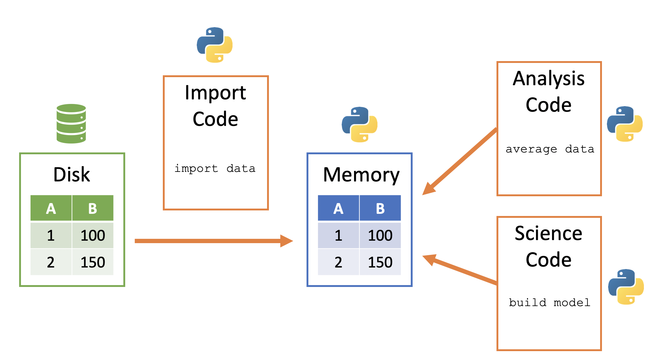
Python stores its data in memory - this makes it relatively quickly accessible but can cause size limitations in certain fields. In this class we will mainly work with small to moderate data sets, which means we should not run into any space limitations.

Note

Python does provide tooling that allows you to work with big data via distributed data (i.e. Pyspark) and relational databrases (i.e. SQL).

Python memory is session-specific, so quitting Python (i.e. shutting down JupyterLab) removes the data from memory. A general way to conceptualize data import into and use within Python:

1. Data sits in on the computer/server - this is frequently called “disk”

2. Python code can be used to copy a data file from disk to the Python session’s memory

3. Python data then sits within Python’s memory ready to be used by other Python code

Here is a visualization of this process:

Delimited files

Video 🎥:

Text files are a popular way to hold and exchange tabular data as almost any data application supports exporting data to the CSV (or other text file) format. Text file formats use delimiters to separate the different elements in a line, and each line of data is in its own line in the text file. Therefore, importing different kinds of text files can follow a fairly consistent process once you’ve identified the delimiter.

Although there are other approaches to importing delimited files, Pandas is often the preferred approach as it greatly simplifies the proess and imports the data directly into a DataFrame – the data structure of choice for tabular data in Python.

The read_csv function is used to import a tabular data file, a CSV, into a DataFrame. The following will import a data set describing the sale of individual residential property in Ames, Iowa from 2006 to 2010 (source).

import pandas as pd

ames = pd.read_csv('../data/ames_raw.csv')

We see that our imported data is represented as a DataFrame:

type(ames)

pandas.core.frame.DataFrame

We can look at it in the Jupyter notebook, since Jupyter will display it in a well-organized, pretty way.

ames

	Order	PID	MS SubClass	MS Zoning	Lot Frontage	Lot Area	Street	Alley	Lot Shape	Land Contour	...	Pool Area	Pool QC	Fence	Misc Feature	Misc Val	Mo Sold	Yr Sold	Sale Type	Sale Condition	SalePrice
0	1	526301100	20	RL	141.0	31770	Pave	NaN	IR1	Lvl	...	0	NaN	NaN	NaN	0	5	2010	WD	Normal	215000
1	2	526350040	20	RH	80.0	11622	Pave	NaN	Reg	Lvl	...	0	NaN	MnPrv	NaN	0	6	2010	WD	Normal	105000
2	3	526351010	20	RL	81.0	14267	Pave	NaN	IR1	Lvl	...	0	NaN	NaN	Gar2	12500	6	2010	WD	Normal	172000
3	4	526353030	20	RL	93.0	11160	Pave	NaN	Reg	Lvl	...	0	NaN	NaN	NaN	0	4	2010	WD	Normal	244000
4	5	527105010	60	RL	74.0	13830	Pave	NaN	IR1	Lvl	...	0	NaN	MnPrv	NaN	0	3	2010	WD	Normal	189900
...	...	...	...	...	...	...	...	...	...	...	...	...	...	...	...	...	...	...	...	...	...
2925	2926	923275080	80	RL	37.0	7937	Pave	NaN	IR1	Lvl	...	0	NaN	GdPrv	NaN	0	3	2006	WD	Normal	142500
2926	2927	923276100	20	RL	NaN	8885	Pave	NaN	IR1	Low	...	0	NaN	MnPrv	NaN	0	6	2006	WD	Normal	131000
2927	2928	923400125	85	RL	62.0	10441	Pave	NaN	Reg	Lvl	...	0	NaN	MnPrv	Shed	700	7	2006	WD	Normal	132000
2928	2929	924100070	20	RL	77.0	10010	Pave	NaN	Reg	Lvl	...	0	NaN	NaN	NaN	0	4	2006	WD	Normal	170000
2929	2930	924151050	60	RL	74.0	9627	Pave	NaN	Reg	Lvl	...	0	NaN	NaN	NaN	0	11	2006	WD	Normal	188000

2930 rows × 82 columns

This is a nice representation of the data, but we really do not need to display that many rows of the DataFrame in order to understand its structure. Instead, we can use the head() method of data frames to look at the first few rows. This is more manageable and gives us an overview of what the columns are. Note also the the missing data was populated with NaN.

ames.head()

	Order	PID	MS SubClass	MS Zoning	Lot Frontage	Lot Area	Street	Alley	Lot Shape	Land Contour	...	Pool Area	Pool QC	Fence	Misc Feature	Misc Val	Mo Sold	Yr Sold	Sale Type	Sale Condition	SalePrice
0	1	526301100	20	RL	141.0	31770	Pave	NaN	IR1	Lvl	...	0	NaN	NaN	NaN	0	5	2010	WD	Normal	215000
1	2	526350040	20	RH	80.0	11622	Pave	NaN	Reg	Lvl	...	0	NaN	MnPrv	NaN	0	6	2010	WD	Normal	105000
2	3	526351010	20	RL	81.0	14267	Pave	NaN	IR1	Lvl	...	0	NaN	NaN	Gar2	12500	6	2010	WD	Normal	172000
3	4	526353030	20	RL	93.0	11160	Pave	NaN	Reg	Lvl	...	0	NaN	NaN	NaN	0	4	2010	WD	Normal	244000
4	5	527105010	60	RL	74.0	13830	Pave	NaN	IR1	Lvl	...	0	NaN	MnPrv	NaN	0	3	2010	WD	Normal	189900

5 rows × 82 columns

File paths

Video 🎥:

It’s important to understand where files exist on your computer and how to reference those paths. There are two main approaches:

1. Absolute paths

2. Relative paths

An absolute path always contains the root elements and the complete list of directories to locate the specific file or folder. For the ames_raw.csv file, the absolute path on my computer is:

import os

absolute_path = os.path.abspath('../data/ames_raw.csv')
absolute_path

'/Users/b294776/Desktop/workspace/training/UC/uc-bana-6043/book/data/ames_raw.csv'

I can always use the absolute path in pd.read_csv():

ames = pd.read_csv(absolute_path)

In contrast, a relative path is a path built starting from the current location. For example, say that I am operating in a directory called “Project A”. If I’m working in “my_notebook.ipynb” and I have a “my_data.csv” file in that same directory:

# illustration of the directory layout
Project A
├── my_notebook.ipynb
└── my_data.csv

Then I can use this relative path to import this file: pd.read_csv('my_data.csv'). This just means to look for the ‘my_data.csv’ file relative to the current directory that I am in.

Often, people store data in a “data” directory. If this directory is a subdirectory within my Project A directory:

# illustration of the directory layout
Project A
├── my_notebook.ipynb
└── data
    └── my_data.csv

Then I can use this relative path to import this file: pd.read_csv('data/my_data.csv'). This just means to look for the ‘data’ subdirectory relative to the current directory that I am in and then look for the ‘my_data.csv’ file.

Sometimes, the data directory may not be in the current directory. Sometimes a project directory will look the following where there is a subdirectory containing multiple notebooks and then another subdirectory containing data assets. If you are working in “notebook1.ipynb” within the notebooks subdirectory, you will need to tell Pandas to go up one directory relative to the notebook you are working in to the main Project A directory and then go down into the data directory.

# illustration of the directory layout
Project A
├── notebooks
│   ├── notebook1.ipynb
│   ├── notebook2.ipynb
│   └── notebook3.ipynb
└── data
    └── my_data.csv

I can do this by using dot-notation in my relative path specification - here I use ‘..’ to imply “go up one directory relative to my current location”: pd.read_csv('../data/my_data.csv').

Note that the path specified in pd.read_csv() does not need to be a local path. For example, the ames_raw.csv data is located online at https://raw.githubusercontent.com/bradleyboehmke/uc-bana-6043/main/book/data/ames_raw.csv. We can use pd.read_csv() to import directly from this location:

url = 'https://raw.githubusercontent.com/bradleyboehmke/uc-bana-6043/main/book/data/ames_raw.csv'
ames = pd.read_csv(url)

Metadata

Once we’ve imported the data we can get some descriptive metadata about our DataFrame. For example, we can get the dimensions of our DataFrame. Here, we see that we have 2,930 rows and 82 columns.

ames.shape

(2930, 82)

We can also see what type of data each column is. For example, we see that the first three columns (Order, PID, MS SubClass) are integers, the fourth column (MS Zoning) is an object, and the fifth (Lot Frontage) is a float.

ames.dtypes

Order               int64
PID                 int64
MS SubClass         int64
MS Zoning          object
Lot Frontage      float64
                   ...   
Mo Sold             int64
Yr Sold             int64
Sale Type          object
Sale Condition     object
SalePrice           int64
Length: 82, dtype: object

The following are the most common data types that appear frequently in DataFrames.

• boolean - only two possible values, True and False

• integer - whole numbers without decimals

• float - numbers with decimals

• object - typically strings, but may contain any object

• datetime - a specific date and time with nanosecond precision

Note

Booleans, integers, floats, and datetimes all use a particular amount of memory for each of their values. The memory is measured in bits. The number of bits used for each value is the number appended to the end of the data type name. For instance, integers can be either 8, 16, 32, or 64 bits while floats can be 16, 32, 64, or 128. A 128-bit float column will show up as float128. Technically a float128 is a different data type than a float64 but generally you will not have to worry about such a distinction as the operations between different float columns will be the same.

We can also use the info() method, which provides output similar to dtypes, but also shows the number of non-missing values in each column along with more info such as:

• Type of object (always a DataFrame)

• The type of index and number of rows

• The number of columns

• The data types of each column and the number of non-missing (a.k.a non-null)

• The frequency count of all data types

• The total memory usage

ames.info()

<class 'pandas.core.frame.DataFrame'>
RangeIndex: 2930 entries, 0 to 2929
Data columns (total 82 columns):
 #   Column           Non-Null Count  Dtype  
---  ------           --------------  -----  
 0   Order            2930 non-null   int64  
 1   PID              2930 non-null   int64  
 2   MS SubClass      2930 non-null   int64  
 3   MS Zoning        2930 non-null   object 
 4   Lot Frontage     2440 non-null   float64
 5   Lot Area         2930 non-null   int64  
 6   Street           2930 non-null   object 
 7   Alley            198 non-null    object 
 8   Lot Shape        2930 non-null   object 
 9   Land Contour     2930 non-null   object 
 10  Utilities        2930 non-null   object 
 11  Lot Config       2930 non-null   object 
 12  Land Slope       2930 non-null   object 
 13  Neighborhood     2930 non-null   object 
 14  Condition 1      2930 non-null   object 
 15  Condition 2      2930 non-null   object 
 16  Bldg Type        2930 non-null   object 
 17  House Style      2930 non-null   object 
 18  Overall Qual     2930 non-null   int64  
 19  Overall Cond     2930 non-null   int64  
 20  Year Built       2930 non-null   int64  
 21  Year Remod/Add   2930 non-null   int64  
 22  Roof Style       2930 non-null   object 
 23  Roof Matl        2930 non-null   object 
 24  Exterior 1st     2930 non-null   object 
 25  Exterior 2nd     2930 non-null   object 
 26  Mas Vnr Type     1155 non-null   object 
 27  Mas Vnr Area     2907 non-null   float64
 28  Exter Qual       2930 non-null   object 
 29  Exter Cond       2930 non-null   object 
 30  Foundation       2930 non-null   object 
 31  Bsmt Qual        2850 non-null   object 
 32  Bsmt Cond        2850 non-null   object 
 33  Bsmt Exposure    2847 non-null   object 
 34  BsmtFin Type 1   2850 non-null   object 
 35  BsmtFin SF 1     2929 non-null   float64
 36  BsmtFin Type 2   2849 non-null   object 
 37  BsmtFin SF 2     2929 non-null   float64
 38  Bsmt Unf SF      2929 non-null   float64
 39  Total Bsmt SF    2929 non-null   float64
 40  Heating          2930 non-null   object 
 41  Heating QC       2930 non-null   object 
 42  Central Air      2930 non-null   object 
 43  Electrical       2929 non-null   object 
 44  1st Flr SF       2930 non-null   int64  
 45  2nd Flr SF       2930 non-null   int64  
 46  Low Qual Fin SF  2930 non-null   int64  
 47  Gr Liv Area      2930 non-null   int64  
 48  Bsmt Full Bath   2928 non-null   float64
 49  Bsmt Half Bath   2928 non-null   float64
 50  Full Bath        2930 non-null   int64  
 51  Half Bath        2930 non-null   int64  
 52  Bedroom AbvGr    2930 non-null   int64  
 53  Kitchen AbvGr    2930 non-null   int64  
 54  Kitchen Qual     2930 non-null   object 
 55  TotRms AbvGrd    2930 non-null   int64  
 56  Functional       2930 non-null   object 
 57  Fireplaces       2930 non-null   int64  
 58  Fireplace Qu     1508 non-null   object 
 59  Garage Type      2773 non-null   object 
 60  Garage Yr Blt    2771 non-null   float64
 61  Garage Finish    2771 non-null   object 
 62  Garage Cars      2929 non-null   float64
 63  Garage Area      2929 non-null   float64
 64  Garage Qual      2771 non-null   object 
 65  Garage Cond      2771 non-null   object 
 66  Paved Drive      2930 non-null   object 
 67  Wood Deck SF     2930 non-null   int64  
 68  Open Porch SF    2930 non-null   int64  
 69  Enclosed Porch   2930 non-null   int64  
 70  3Ssn Porch       2930 non-null   int64  
 71  Screen Porch     2930 non-null   int64  
 72  Pool Area        2930 non-null   int64  
 73  Pool QC          13 non-null     object 
 74  Fence            572 non-null    object 
 75  Misc Feature     106 non-null    object 
 76  Misc Val         2930 non-null   int64  
 77  Mo Sold          2930 non-null   int64  
 78  Yr Sold          2930 non-null   int64  
 79  Sale Type        2930 non-null   object 
 80  Sale Condition   2930 non-null   object 
 81  SalePrice        2930 non-null   int64  
dtypes: float64(11), int64(28), object(43)
memory usage: 1.8+ MB

Attributes & methods

Video 🎥:

We’ve seen that we can use the dot-notation to access functions in libraries (i.e. pd.read_csv()). We can use this same approach to access things inside of objects. What’s an object? Basically, a variable that contains other data or functionality inside of it that is exposed to users. Consequently, our DataFrame item is an object.

In the above code, we saw that we can make different calls with our DataFrame such as ames.shape and ames.head(). An observant reader probably noticed the difference between the two – one has parentheses and the other does not.

An attribute inside an object is simply a variable that is unique to that object and a method is just a function inside an object that is unique to that object.

Tip

Variables inside an object are often called attributes and functions inside objects are called methods.

attribute: A variable associated with an object and is referenced by name using dotted expressions. For example, if an object o has an attribute a it would be referenced as o.a

method: A function associated with an object and is also referenced using dotted expressions but will include parentheses. For example, if an object o has a method m it would be called as o.m()

Earlier, we saw the attributes shape and dtypes. Another attribute is columns, which will list all column names in our DataFrame.

ames.columns

Index(['Order', 'PID', 'MS SubClass', 'MS Zoning', 'Lot Frontage', 'Lot Area',
       'Street', 'Alley', 'Lot Shape', 'Land Contour', 'Utilities',
       'Lot Config', 'Land Slope', 'Neighborhood', 'Condition 1',
       'Condition 2', 'Bldg Type', 'House Style', 'Overall Qual',
       'Overall Cond', 'Year Built', 'Year Remod/Add', 'Roof Style',
       'Roof Matl', 'Exterior 1st', 'Exterior 2nd', 'Mas Vnr Type',
       'Mas Vnr Area', 'Exter Qual', 'Exter Cond', 'Foundation', 'Bsmt Qual',
       'Bsmt Cond', 'Bsmt Exposure', 'BsmtFin Type 1', 'BsmtFin SF 1',
       'BsmtFin Type 2', 'BsmtFin SF 2', 'Bsmt Unf SF', 'Total Bsmt SF',
       'Heating', 'Heating QC', 'Central Air', 'Electrical', '1st Flr SF',
       '2nd Flr SF', 'Low Qual Fin SF', 'Gr Liv Area', 'Bsmt Full Bath',
       'Bsmt Half Bath', 'Full Bath', 'Half Bath', 'Bedroom AbvGr',
       'Kitchen AbvGr', 'Kitchen Qual', 'TotRms AbvGrd', 'Functional',
       'Fireplaces', 'Fireplace Qu', 'Garage Type', 'Garage Yr Blt',
       'Garage Finish', 'Garage Cars', 'Garage Area', 'Garage Qual',
       'Garage Cond', 'Paved Drive', 'Wood Deck SF', 'Open Porch SF',
       'Enclosed Porch', '3Ssn Porch', 'Screen Porch', 'Pool Area', 'Pool QC',
       'Fence', 'Misc Feature', 'Misc Val', 'Mo Sold', 'Yr Sold', 'Sale Type',
       'Sale Condition', 'SalePrice'],
      dtype='object')

Similar to regular functions, methods are called with parentheses and often take arguments. For example, we can use the tail() method to see the last n rows in our DataFrame:

ames.tail(3)

	Order	PID	MS SubClass	MS Zoning	Lot Frontage	Lot Area	Street	Alley	Lot Shape	Land Contour	...	Pool Area	Pool QC	Fence	Misc Feature	Misc Val	Mo Sold	Yr Sold	Sale Type	Sale Condition	SalePrice
2927	2928	923400125	85	RL	62.0	10441	Pave	NaN	Reg	Lvl	...	0	NaN	MnPrv	Shed	700	7	2006	WD	Normal	132000
2928	2929	924100070	20	RL	77.0	10010	Pave	NaN	Reg	Lvl	...	0	NaN	NaN	NaN	0	4	2006	WD	Normal	170000
2929	2930	924151050	60	RL	74.0	9627	Pave	NaN	Reg	Lvl	...	0	NaN	NaN	NaN	0	11	2006	WD	Normal	188000

3 rows × 82 columns

Note

We will be exposed to many of the available DataFrame methods throughout this course!

Knowledge check

Questions:

1. Check out the help documentation for read_csv() by executing pd.read_csv? in a code cell. What parameter in read_csv() allows us to specify values that represent missing values?

2. Read in this energy_consumption.csv file.

3. What are the dimesions of this data? What information does the size attribute provide?

4. Check out the describe() method. What information does this provide?

Excel files

With Excel still being the spreadsheet software of choice its important to be able to efficiently import and export data from these files. Often, users will simply resort to exporting the Excel file as a CSV file and then import into Python using pandas.read_csv; however, this is far from efficient. This section will teach you how to eliminate the CSV step and to import data directly from Excel using pandas’ built-in read_excel() function.

To illustrate, we’ll import so mock grocery store products data located in a products.xlsx file.

Note

You may need to install the openpyxl dependency. You can do so with either of the following:

• pip install openpyxl

• conda install openpyxl

To read in Excel data with pandas, you will use the ExcelFile() and read_excel() functions. ExcelFile allows you to read the names of the different worksheets in the Excel workbook. This allows you to identify the specific worksheet of interest and then specify that in read_excel.

products_excel = pd.ExcelFile('../data/products.xlsx')
products_excel.sheet_names

['metadata', 'products data', 'grocery list']

Warning

If you don’t explicitly specify a sheet then the first worksheet will be imported.

products = pd.read_excel('../data/products.xlsx', sheet_name='products data')
products.head()

	product_num	department	commodity	brand_ty	x5
0	92993	NON-FOOD	PET	PRIVATE	N
1	93924	NON-FOOD	PET	PRIVATE	N
2	94272	NON-FOOD	PET	PRIVATE	N
3	94299	NON-FOOD	PET	PRIVATE	N
4	94594	NON-FOOD	PET	PRIVATE	N

SQL databases

Many organizations continue to use relational databases along with SQL to interact with these data assets. Python has many tools to interact with these databases and you can even query SQL database tables with Panda’s read_sql command. Pandas relies on a third-party library called SQLAlechmy to establish a connection to a database.

To connect to a database, we need to pass a connection string to SQLAlechmy’s create_engine() function. The general form of a connection string is the following: dialect+driver://username:password@host:port/database.

Note

Read more about engine configuration here.

In this example I will illustrate connecting to a local sqlite database. To do so the connection string looks like: sqlite:///<path_to_db>. The following illustrates with the example Chinook Database, which I’ve downloaded to my data directory.

from sqlalchemy import create_engine

engine = create_engine('sqlite:///../data/chinook.db')

Once I’ve made the connection, I can use pd.read_sql() to read in the “tracks” table directly as a Pandas DataFrame.

tracks = pd.read_sql('tracks', con=engine)
tracks.head()

	TrackId	Name	AlbumId	MediaTypeId	GenreId	Composer	Milliseconds	Bytes	UnitPrice
0	1	For Those About To Rock (We Salute You)	1	1	1	Angus Young, Malcolm Young, Brian Johnson	343719	11170334	0.99
1	2	Balls to the Wall	2	2	1	None	342562	5510424	0.99
2	3	Fast As a Shark	3	2	1	F. Baltes, S. Kaufman, U. Dirkscneider & W. Ho...	230619	3990994	0.99
3	4	Restless and Wild	3	2	1	F. Baltes, R.A. Smith-Diesel, S. Kaufman, U. D...	252051	4331779	0.99
4	5	Princess of the Dawn	3	2	1	Deaffy & R.A. Smith-Diesel	375418	6290521	0.99

If you are familiar with SQL then you can even pass a SQL query directly in the pd.read_sql() call. For example, the following SQL query:

1. SELECTS the name, composer, and milliseconds columns,

2. FROM the tracks table,

3. WHERE observations in the milliseconds column are greater than 200,000 and WHERE observations in the composer column are not missing (NULL)

sql_query = '''SELECT name, composer, milliseconds
               FROM tracks
               WHERE milliseconds > 200000 and composer is not null'''

long_tracks = pd.read_sql(sql_query, engine)
long_tracks.head()

	Name	Composer	Milliseconds
0	For Those About To Rock (We Salute You)	Angus Young, Malcolm Young, Brian Johnson	343719
1	Fast As a Shark	F. Baltes, S. Kaufman, U. Dirkscneider & W. Ho...	230619
2	Restless and Wild	F. Baltes, R.A. Smith-Diesel, S. Kaufman, U. D...	252051
3	Princess of the Dawn	Deaffy & R.A. Smith-Diesel	375418
4	Put The Finger On You	Angus Young, Malcolm Young, Brian Johnson	205662

Many other file types

There are many other file types that you may encounter in your career. Most of which we can import into Python one way or another. Most tabular (2-dimensional data sets) can be imported directly with Pandas. For example, this page shows a list of the many pandas.read_xxx() functions that allow you to read various data file types.

While tabular data is the most popular in data science, other types of data will are used as well. These are not as important as the pandas DataFrame, but it is good to be exposed to them. These additional data formats are going to be more common in a fully functional programming language like Python.

JSON files

A common example is a JSON file – these are non-tabular data files that are popular in data engineering due to their space efficiency and flexibility. Here is an example JSON file:

{
    "planeId": "1xc2345g",
    "manufacturerDetails": {
        "manufacturer": "Airbus",
        "model": "A330",
        "year": 1999
    },
    "airlineDetails": {
        "currentAirline": "Southwest",
        "previousAirlines": {
            "1st": "Delta"
        },
        "lastPurchased": 2013
    },
    "numberOfFlights": 4654
}

Note

Does this JSON data structure remind you of a Python data structure? The JSON file bears a striking resemblance to the Python dictionary structure due to the key-value pairings.

JSON Files can be imported using the json library (from the Standard library) paired with the with statement and the open() function.

import json

with open('../data/json_example.json', 'r') as f:
    imported_json = json.load(f)

We can then verify that our imported object is a dict:

type(imported_json)

dict

And we can view the data:

imported_json

{'planeId': '1xc2345g',
 'manufacturerDetails': {'manufacturer': 'Airbus',
  'model': 'A330',
  'year': 1999},
 'airlineDetails': {'currentAirline': 'Southwest',
  'previousAirlines': {'1st': 'Delta'},
  'lastPurchased': 2013},
 'numberOfFlights': 4654}

Pickle files

So far, we’ve seen that tabular data files can be imported and represented as DataFrames and JSON files can be imported and represented as dicts, but what about other, more complex data?

Python’s native data files are known as Pickle files:

• All Pickle files have the .pickle extension

• Pickle files are great for saving native Python data that can’t easily be represented by other file types such as:

  • pre-processed data,

  • models,

  • any other Python object…

Similar to JSON files, pickle files can be imported using the pickle library paired with the with statement and the open() function:

import pickle

with open('../data/pickle_example.pickle', 'rb') as f:
    imported_pickle = pickle.load(f)

We can view this file and see it’s the same data as the JSON:

imported_pickle

{'planeId': '1xc2345g',
 'manufacturerDetails': {'manufacturer': 'Airbus',
  'model': 'A330',
  'year': 1999},
 'airlineDetails': {'currentAirline': 'Southwest',
  'previousAirlines': {'1st': 'Delta'},
  'lastPurchased': 2013},
 'numberOfFlights': 4654}

Additional video tutorial

Video 🎥:

Here’s an additional video provided by Corey Schafer that you might find useful. It covers importing and exporting data from multiple different sources.

Exercises

Questions:

1. Python stores its data in _______ .

2. What happens to Python’s data when the Python session is terminated?

3. Load the hearts.csv data file into Python using the pandas library.

4. What are the dimensions of this data? What data types are the variables in this data set?

5. Assess the first 10 rows of this data set.

6. Now import the hearts_data_dictionary.csv file, which provides some information on each variable. Do the data types of the hearts.csv variables align with the description of each variable?

Computing environment

Show code cell source Hide code cell source

%load_ext watermark
%watermark -v -p jupyterlab,pandas,sqlalchemy

Python implementation: CPython
Python version       : 3.12.4
IPython version      : 8.26.0

jupyterlab: 4.2.3
pandas    : 2.2.2
sqlalchemy: 2.0.31