Lesson 1a: Introduction to JupyterLab

---

In this lesson we will introduce the Python interpreter along with JupyterLab and notebooks.

Learning objectives

By the end of this lesson you will be able to:

• Open and execute code in the JupyterLab console.

• Execute a simple .py file from the terminal and console within JupyterLab.

• Explain the benefits of a Jupyter notebook and create code and markdown cells.

The Python interpreter

Before diving into the Python interpreter, I pause here to remind you that this class is not meant to teach Python syntax (though you will learn plenty of that!). The things you learn here are meant to help you understand, and ultimately do, statistical computing more generally. Think of it this way: this class is meant to help you unleash the power of your computer on your statistical problems. Python is just the language of instruction. That said, let’s start talking about how Python works.

Python is an interpreted language, which means that each line of code you write is translated, or interpreted, into a set of instructions that your machine can understand by the Python interpreter. This stands in contrast to compiled languages. For these languages (the dominant ones being Fortran, C, and C++), your entire code is translated into machine language before you ever run it. When you execute your program, it is already in machine language.

So, whenever you want your Python code to run, you give it to the Python interpreter.

There are many ways to launch the Python interpreter. One way is to type

python

on the command line of a terminal. This launches the vanilla Python interpreter. We will never really use this in this class. Rather, we will have a greatly enhanced Python experience, either using IPython, a feature-rich, enhanced interactive Python available through JupyterLab’s console, or using a notebook, also launchable in JupyterLab.

Hello, world. and the print() function

Traditionally, the first program anyone writes when learning a new language is called “Hello, world.” In this program, the words “Hello, world.” are printed on the screen. The original Hello, world. was likely written by Brian Kernighan, one of the inventors of Unix, and the author of the classic and authoritative book on the C programming language. In his original, the printed text was “hello, world” (no period or capital H), but people use lots of variants.

We will first write and run this little program using a JupyterLab console. After launching JupyterLab, you probably already have the Launcher in your JupyterLab window. If you do not, you can expand the Files tab at the left of your JupyterLab window (if it is not already expanded) by clicking on that tab, or alternatively hit ctrl+b (or cmd+b on macOS). At the top of the Files tab is a + sign, which gives you a Jupyter Launcher.

In the Jupyter Launcher, click the Python 3 icon under Console. This will launch a console, which has a large white space above a prompt that says In []:. You can enter Python code in this prompt, and it will be executed.

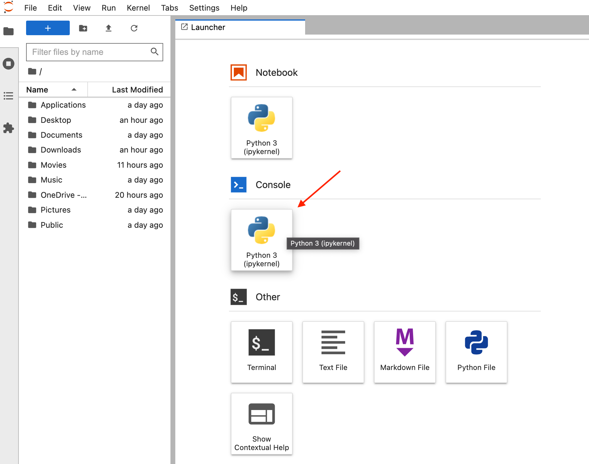
Fig. 4 Launch the IPython console.

To print Hello, world., enter the code below. To execute the code, hit shift+enter.

print('Hello, world.')

Hello, world.

Hooray! We just printed Hello, world. to the screen. To do this, we used Python’s built-in print() function. The print() function takes as an argument a string. It then prints that string to the screen. We will learn more about function syntax later, but we can already see the rough syntax with the print() function.

Video 🎥:

.py files

Now let’s use our new knowledge of the print() function to have our computer say a bit more than just Hello, world. Type these lines in at the prompt, hitting enter each time you need a new line. After you’ve typed them all in, hit shift+enter to run them.

# The first few lines from The Zen of Python by Tim Peters
print('Beautiful is better than ugly.')
print('Explicit is better than implicit.')
print('Simple is better than complex.')
print('Complex is better than complicated.')

Beautiful is better than ugly.
Explicit is better than implicit.
Simple is better than complex.
Complex is better than complicated.

Note that the first line is preceded with a # sign, and the Python interpreter ignored it. The # sign denotes a comment, which is ignored by the interpreter, but very very important for the human!

While the console prompt was nice entering all of this, an alternative option is to store them in a file, and then have the Python interpreter run the lines in the file. This is how you typically store Python code, and the suffix of such files is .py.

So, let’s create a .py file. To do this, use the JupyterLab Launcher to launch a Python file.

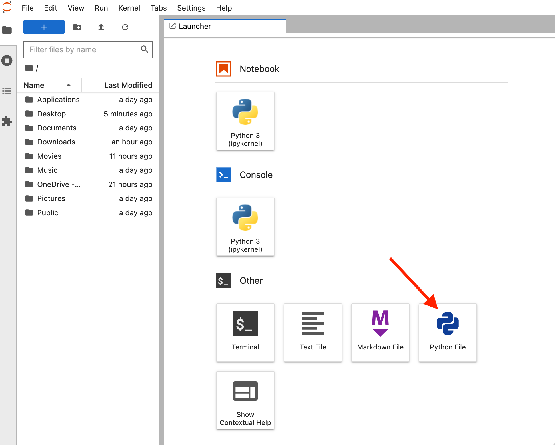
Fig. 5 Create a Python file.

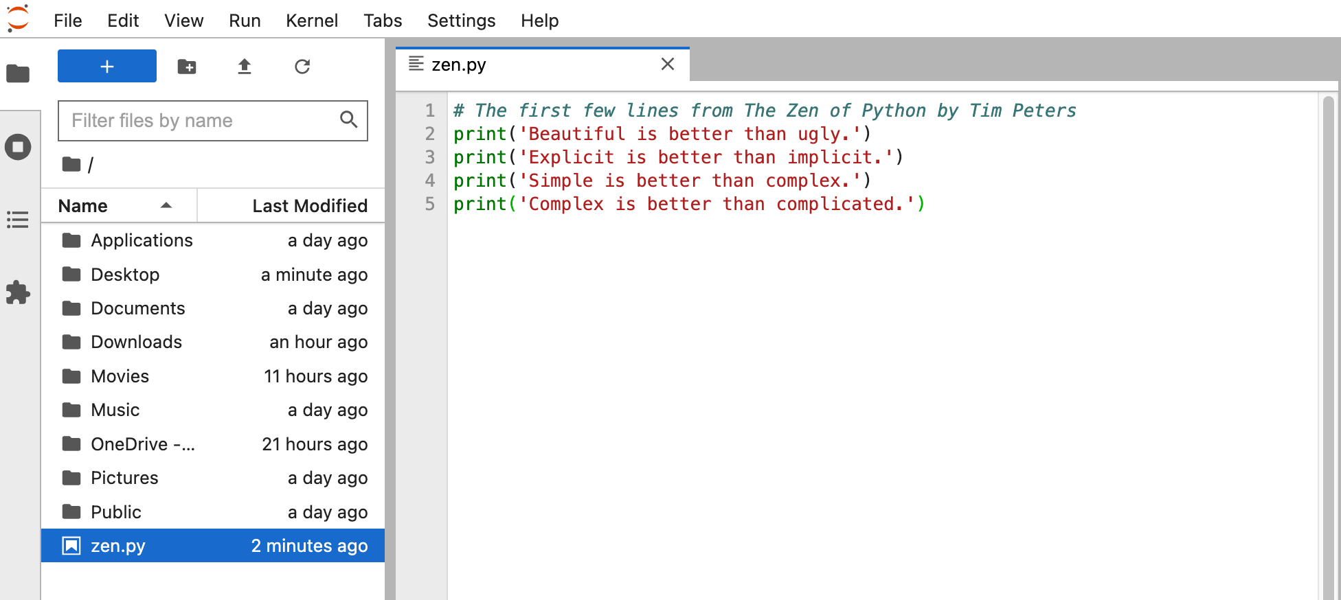
Once it is launched, you can right click on the tab of the text editor window to change the name. We will call this file zen.py. Within this file, enter the four lines of code you previously entered in the console prompt. Be sure to save it; it should look as below:

Fig. 6 Example zen.py file.

To run the code in this file, you can invoke the Python interpreter at the command line, followed by the file name. I.e., enter

python zen.py

at the command line. Note that when you run code this way, the interpreter exits after completion of running the code, and you do not get a prompt.

To run the code in this file using the Jupyter console, you can use the %run magic function.

%run zen.py

Beautiful is better than ugly.
Explicit is better than implicit.
Simple is better than complex.
Complex is better than complicated.

Note

While some Python programmers execute all of their Python code in this “scripting” fashion, those doing data analysis or scientific computing largely make use of Jupyter notebooks. For the majority of this class you will be using Jupyter notebooks but later on you will be exposed to some scripting activities as it is an important skill to have.

To shut down the console, you can click on the Running tab at the left of the JupyterLab window and click on SHUTDOWN next to the console.

Video 🎥:

Jupyter

At this point, we have introduced JupyterLab, its text editor, and the IPython console, as well as the Python interpreter itself. You might be asking….

What is Jupyter?

From the Project Jupyter website:

Project Jupyter is an open source project was born out of the IPython Project in 2014 as it evolved to support interactive data science and scientific computing across all programming languages.

So, Jupyter is an extension of IPython that pushes interactive computing further. It is language agnostic as its name suggests. The name “Jupyter” is a combination of Julia (a new language for scientific computing), Python (which you know and love), and R (another dominant tool for statistical computation). However, you can run over 40 different languages in a JupyterLab, not just Julia, Python, and R.

Central to Jupyter/JupyterLab are Jupyter notebooks. In fact, the document you are reading right now was generated from a Jupyter notebook. We will use Jupyter notebooks extensively in this class, along with .py files and the console.

Why Jupyter notebooks?

When writing code you will reuse or productionize, you will usually develop fully tested modules using .py files. You can always import those modules when you are using a Jupyter notebook (more on modules and importing them later in the class). Consequently, a Jupyter notebook is often not optimal for an application where you are building reusable code or scripts or productionizing code. However, Jupyter notebooks are very useful in the following applications.

1. Exploratory data analysis. Jupyter notebooks are great for trying things out with code, or exploring a data set. This is an important part of the research process. The layout of Jupyter notebooks is great for organizing thoughts as you synthesize them.

2. Developing visualizations. This is really just a special case of (1), but is worth mentioning separately because Jupyter notebooks are especially useful when interactively visualizing data. Using the Jupyter notebook, you can write down what you hope to accomplish in each step of processing and then graphically show the results with plots as you go through the analysis. We will do this later in the class.

3. Sharing your thinking in your analysis. Because you can combine nicely formatted text and executable code, Jupyter notebooks are great for sharing how you go about doing your calculations with collaborators and with readers of your publications.

4. Pedagogy. All of the content in this class, including this lesson, was developed using Jupyter notebooks! You will find lots of educational content online that is developed and hosted directly in Jupyter notebooks.

Now that we know what Jupyter notebooks are and what the motivation is for using them, let’s start!

Launching a Jupyter notebook

To launch a Jupyter notebook, click on the Notebook icon of the JupyterLab launcher. If you want to open an existing notebook, right click on it in the Files tab of the JupyterLab window and open it.

Modes

At this point you are presented with a notebook with an empty cell.

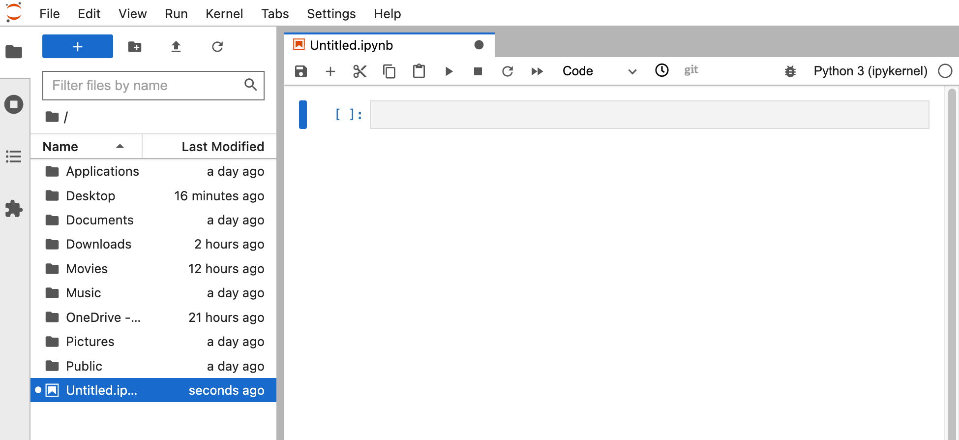
Fig. 7 Initial view of an empty Jupyter notebook.

A notebook consists of two modes - command mode and edit mode. Command mode is for creating and manipulating cells while edit mode is for changing what is inside of a single cell. You will know what mode you are in because when you are in edit mode, the cell you are in will be blue. For both modes there are many keyboard shortcuts that you will learn over time.

Tip

If you are in command mode you can use the keyboard shortcut enter to move into a cell and go into edit mode.

If you are inside a cell and in edit mode you can jump out of the cell into command mode with the esc keyboard shortcut.

Cells

A Jupyter notebook consists of cells. The two main types of cells you will use are code cells and markdown cells, and we will go into their properties in depth momentarily. First, an overview.

A code cell contains actual code that you want to run. You can specify a cell as a code cell using the “Code” pulldown menu in the toolbar of your Jupyter notebook. Otherwise, you can can hit y while a cell is selected and you are in command mode to specify that it is a code cell. Note that you will have to hit enter after doing this to start editing it.

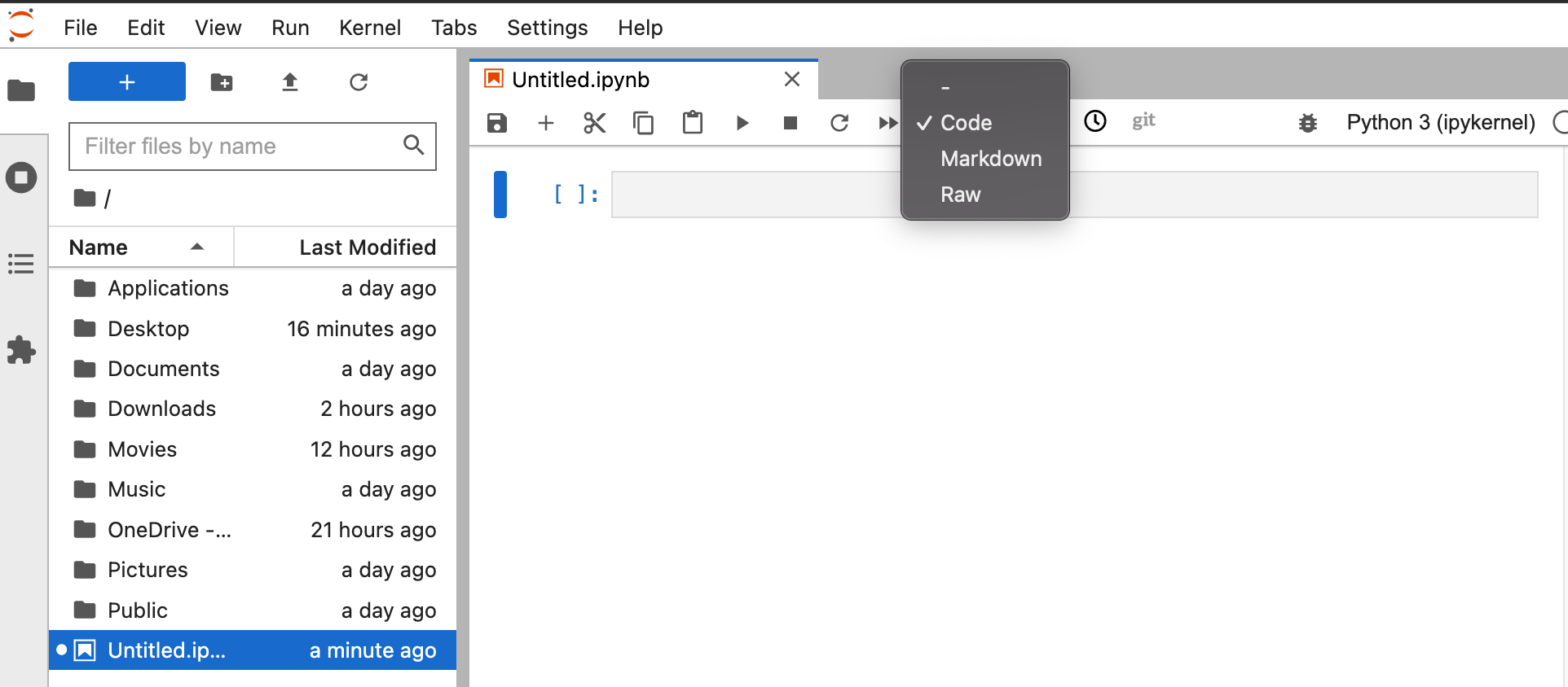
Fig. 8 Change a cell type.

If you want to execute the code in a code cell, hit Enter while holding down the Shift key (denoted Shift + Enter). Note that code cells are executed in the order you shift-enter them. That is to say, the ordering of the cells for which you hit Shift + Enter is the order in which the code is executed. If you did not explicitly execute a cell early in the document, its results are not known to the Python interpreter. This is a very important point and is often a source of confusion and frustration for students.

Markdown cells contain text. The text is written in markdown, a lightweight markup language. You can read about its syntax here. Note that you can also insert HTML into markdown cells, and this will be rendered properly. As you are typing the contents of these cells, the results appear as text. Hitting Shift + Enter renders the text in the formatting you specify.

You can specify a cell as being a markdown cell in the Jupyter toolbar, or by hitting m while a cell is selected and you are in command mode. Again, you have to hit enter after using the quick keys to bring the cell into edit mode.

In general, when you want to add a new cell, you can click the + icon on the notebook toolbar. The shortcut to insert a cell below your current location is b and to insert a cell above is a. Alternatively, you can execute a cell and automatically add a new one below it by hitting Alt + Enter.

Code cells

Below is an example of a code cell printing hello, world. Notice that the output of the print statement appears in the same cell, though separate from the code block.

# Say hello to the world.
print('hello, world.')

hello, world.

If you evaluate a Python expression that returns a value, that value is displayed as output of the code cell. This only happens, however, for the last line of the code cell.

# Would show 9 if this were the last line, but it is not, so shows nothing
4 + 5

# I hope we see 11.
5 + 6

11

Note, however, if the last line does not return a value, such as if we assigned value to a variable, there is no visible output from the code cell.

# Variable assignment, so no visible output.
a = 5 + 6

# However, now if we ask for a, its value will be displayed
a

11

Display of graphics

When we learn about plotting with Seaborn, Bokeh and HoloViews later in this class, you will learn about displaying graphics in Jupyter notebooks.

Quick keys

There are some keyboard shortcuts that are convenient to use in JupyterLab. We already encountered several of them. Importantly, pressing Esc brings you into command mode in which you are not editing the contents of a single cell, but are doing things like adding cells. And pressing Enter will take you into a selected cell to edit that particular cell. Below are some useful quick keys. If two keys are separated by a + sign, they are pressed simultaneously, and if they are separated by a - sign, they are pressed in succession.

Table 1 Jupyter notebook keyboard shortcuts

Quick keys	Mode	Action
m	command	switch cell to Markdown cell
y	command	switch cell to code cell
a	command	insert cell above
b	command	insert cell below
d - d	command	delete cell
0 - 0	command	restart kernel
i - i	command	interupt kernel
shift + enter	edit	execute cell and insert a cell below
Cmd\|Alt + Enter	edit	execute cell

There are many others (and they are shown in the pulldown menus within JupyterLab), but these are the ones I seem to encounter most often.

Video 🎥:

Exercises

Questions:

1. Check out the various reference docs located under Help in the Jupyter Lab toolbar.

2. Create or open a notebook in Jupyter.

3. Create a new markdown cell. Write your name in it and execute the cell.

4. Read about the Markdown syntax in the Markdown reference doc (Jupyer Lab toolbar >> Help) and create a new markdown cell that includes:

   • a second-level header

   • an unordered list

   • an ordered list

   • a hyperlink

   • an image

5. Create a new code cell. Write x = 5 and run it.

Additional video

Video 🎥:

Here’s a webinar that provides a nice discussion of Jupyter Lab and Notebooks. It is not necessary to watch this but may help to kickstart your abilities with Jupyter!

Computing environment

At the end of every lesson, and indeed at the end (or beginning) of any notebook you make, we should include information about the computing environment including the version numbers of all packages we use. The watermark package is quite useful for this. The watermark package is an IPython magic extension. These extensions allow convenient functionality within IPython or Jupyter notebooks. In general, to use magic functions, you precede them with a % sign or a %% in a cell. We use the built-in %load_ext magic function to load watermark, and then we use %watermark to invoke it.

We use the -v flag to ask watermark to give us the Python and IPython verison numbers and the -p flag to give us version numbers on specified packages we’ve used. We can also use a -m flag to give information about the machine running the notebook, and you should do that, but I will not do that for the class to avoid clutter.

%load_ext watermark
%watermark -v -p jupyterlab

Python implementation: CPython
Python version       : 3.12.4
IPython version      : 8.26.0

jupyterlab: 4.2.3