Lesson 4b: Relational data

Lesson 4b: Relational data#

It’s rare that a data analysis involves only a single table of data. Typically you have many tables of data, and you must combine them to answer the questions that you’re interested in. Collectively, multiple tables of data are called relational data because its the relations, not just the individual data sets, that are important.

To work with relational data you need join operations that work with pairs of tables. There are several types of join methods to work with relational data and in this lesson we are going to explore these various methods.

Learning objectives#

By the end of this lesson you’ll be able to:

Use various mutating joins to combine variables from two tables.
Join two tables that have differing common key variable names.
Include an indicator variable while joining so you can filter the joined data for follow-on analysis.

Video 🎥:

Here’s a great video discussing ways to join DataFrames. Watch this video for an initial introduction and then get more hands on by working through the lesson that follows.

Prerequisites#

Load Pandas to provide you access to the join functions we’ll cover in this lesson.

import pandas as pd

To illustrate various joining tasks we will use two very simple DataFrames x & y. The colored column represents the “key” variable: these are used to match the rows between the tables. We’ll talk more about keys in a second. The grey column represents the “value” column that is carried along for the ride.

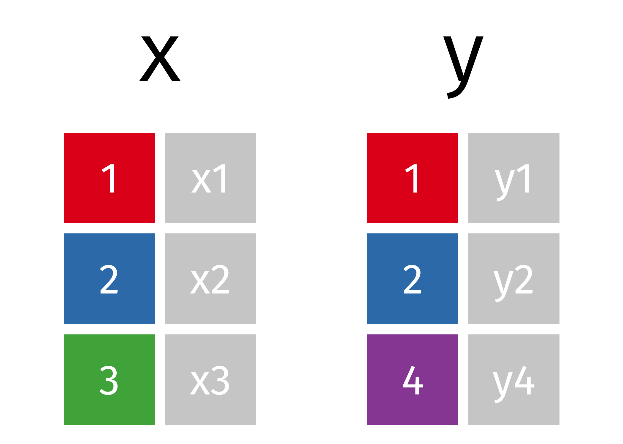
Example DataFrames — Fig. 9 Two simple DataFrames.#

x = pd.DataFrame({'id': [1, 2, 3], 'val_x': ['x1', 'x2', 'x3']})
y = pd.DataFrame({'id': [1, 2, 4], 'val_y': ['y1', 'y2', 'y4']})

However, we will also build upon the simple examples by using various data sets from the completejourney_py library. This library provides access to data sets characterizing household level transactions over one year from a group of 2,469 households who are frequent shoppers at a grocery store.

There are eight built-in data sets available in this library. The data sets include:

campaigns: campaigns received by each household
campaign_descriptions: campaign metadata (length of time active)
coupons: coupon metadata (UPC code, campaign, etc.)
coupon_redemptions: coupon redemptions (household, day, UPC code, campaign)
demographics: household demographic data (age, income, family size, etc.)
products: product metadata (brand, description, etc.)

This is a Python equivalent of the R package completejourney. The R package has a full guide to get you acquainted with the various data set schemas, which you can read here.

from completejourney_py import get_data

# get_data() provides a dictionary of several DataFrames
cj_data = get_data()
cj_data.keys()

dict_keys(['campaign_descriptions', 'coupons', 'promotions', 'campaigns', 'demographics', 'transactions', 'coupon_redemptions', 'products'])

cj_data['transactions'].head()

	household_id	store_id	basket_id	product_id	quantity	sales_value	retail_disc	week	transaction_timestamp
0	900	330	31198570044	1095275	1	0.50	0.00	1	2017-01-01 11:53:26
1	900	330	31198570047	9878513	1	0.99	0.10	1	2017-01-01 12:10:28
2	1228	406	31198655051	1041453	1	1.43	0.15	1	2017-01-01 12:26:30
3	906	319	31198705046	1020156	1	1.50	0.29	1	2017-01-01 12:30:27
4	906	319	31198705046	1053875	2	2.78	0.80	1	2017-01-01 12:30:27

TODO

Take some time to read about the completejourney data set schema here.

What different data sets are available and what do they represent?
What are the common variables between each table?

Keys#

The variables used to connect two tables are called keys. A key is a variable (or set of variables) that uniquely identifies an observation. There are two primary types of keys we’ll consider in this lesson:

A primary key uniquely identifies an observation in its own table
A foreign key uniquely identifies an observation in another table

Variables can be both a primary key and a foreign key. For example, within the transactions data household_id is a primary key to represent a household identifier for each transaction. household_id is also a foreign key in the demographics data set where it can be used to align household demographics to each transaction.

A primary key and the corresponding foreign key in another table form a relation. Relations are typically one-to-many. For example, each transaction has one household, but each household has many transactions. In other data, you’ll occasionally see a 1-to-1 relationship.

When data is cleaned appropriately the keys used to match two tables will be commonly named. For example, the variable that can link our x and y data sets is named id:

x.columns.intersection(y.columns)

Index(['id'], dtype='object')

We can easily see this by looking at the x and y data but when working with larger data sets this becomes more appropriate than just viewing the data. For example, we can easily identify the common columns in the completejourney_py transactions and demographics data:

transactions = cj_data['transactions']
demographics = cj_data['demographics']

transactions.columns.intersection(demographics.columns)

Index(['household_id'], dtype='object')

Note

Although it is preferred, keys do not need to have the same name in both tables. For example, our household identifier could be named household_id in the transaction data but be hshd_id in the demographics table. The names would be different but they represent the same information.

Mutating joins#

Often we have separate DataFrames that can have common and differing variables for similar observations and we wish to join these DataFrames together. A mutating join allows you to combine variables from two tables. It first matches observations by their keys, then copies across variables from one table to the other.

There are different types of joins depending on how you want to merge two DataFrames:

inner join: keeps only observations in x that match in y.
left join: keeps all observations in x and adds available information from y.
right join: keeps all observations in y and adds available information from x.
full join: keeps all observations in both x and y.

Let’s explore each of these a little more closely.

Note

DataFrames have two different methods to join data - df.join() & df.merge(). The .join method is meant for joining based on the index rather than columns. In practice, .merge tends to be used more often because it allows us to retain variables in columns and join by one or more columns. Consequently, we will be using .merge throughout this lesson.

Inner join#

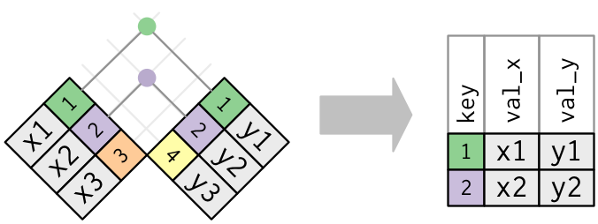
The simplest type of join is the inner join. An inner join matches pairs of observations whenever their keys are equal. Consequently, the output of an inner join is all rows from x where there are matching values in y, and all columns from x and y.

Note

An inner join is the most restrictive of the joins - it returns only rows with matches across both data frames.

The following provides a nice illustration:

To perform an inner join with Pandas we use the .merge method. By default, .merge will perform an inner join:

x.merge(y)

	id	val_x	val_y
0	1	x1	y1
1	2	x2	y2

Note

Notice that only those rows where there are common key values (id = 1 & 2) in both x and y are retained while the rows where non-common key values exist (id = 3 in x and id = 4 in y) are discarded.

Note that I didn’t specify which column to join on nor the type of join. If that information is not specified, merge uses the overlapping column names as the keys. It’s a good practice to specify the type of join and the keys explicitly:

x.merge(y, how='inner', on='id')

	id	val_x	val_y
0	1	x1	y1
1	2	x2	y2

Outer joins#

An inner join keeps observations that appear in both tables. However, we often want to retain all observations in at least one of the tables. Consequently, we can apply various outer joins to retain observations that appear in at least one of the tables. There are three main types of outer joins:

A left join keeps all observations in x.
A right join keeps all observations in y.
A full join keeps all observations in x and y.

These joins work by adding NaN in rows where non-matching information exists:

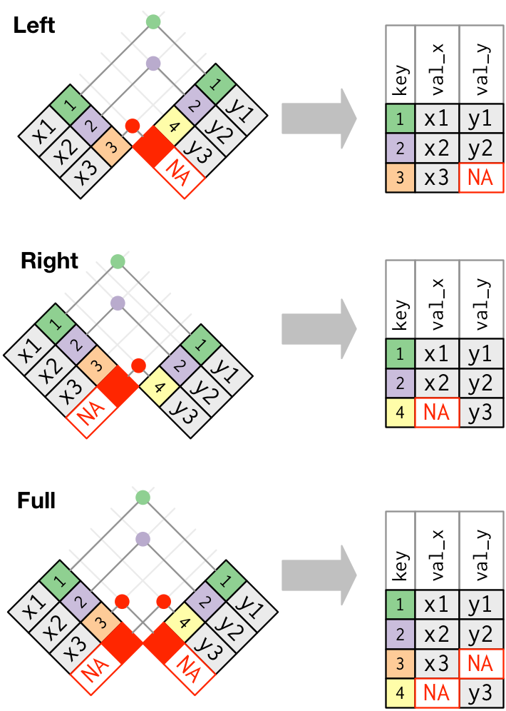
Outer joins — Fig. 11 Difference in left join, right join, and outer join procedures (source).#

Left join#

With a left join we retain all observations from x, and we add columns y. Rows in x where there is no matching key value in y will have NaN values in the new columns. We can change the type of join by changing the how argument.

x.merge(y, how='left', on='id')

	id	val_x	val_y
0	1	x1	y1
1	2	x2	y2
2	3	x3	NaN

Right join#

A right join is just a flipped left join where we retain all observations from y, and we add columns x. Similar to a left join, rows in y where there is no matching key value in x will have NaN values in the new columns.

Note

Should I use a right join, or a left join? To answer this, ask yourself “which DataFrame should retain all of its rows?” - and use this one as the baseline. A left join keeps all the rows in the first DataFrame written in the command, whereas a right join keeps all the rows in the second DataFrame.

x.merge(y, how='right', on='id')

	id	val_x	val_y
0	1	x1	y1
1	2	x2	y2
2	4	NaN	y4

Full outer join#

We can also perform a full outer join where we keep all observations in x and y. This join will match observations where the key variable(s) have matching information in both tables and then fill in non-matching values as NaN.

Note

A full outer join is the most inclusive of the joins - it returns all rows from both DataFrames.

x.merge(y, how='outer', on='id')

	id	val_x	val_y
0	1	x1	y1
1	2	x2	y2
2	3	x3	NaN
3	4	NaN	y4

Differing keys#

So far, the keys we’ve used to join two DataFrames have had the same name. This was encoded by using on='id'. However, having keys with the same name is not a requirement. But what happens we our common key variable is named differently in each DataFrame?

a = pd.DataFrame({'id_a': [1, 2, 3], 'val_a': ['x1', 'x2', 'x3']})
b = pd.DataFrame({'id_b': [1, 2, 4], 'val_b': ['y1', 'y2', 'y4']})

In this case, since our common key variable has different names in each table (id_a in a and id_b in b), our inner join function doesn’t know how to join these two DataFrames and an error results.

a.merge(b)

---------------------------------------------------------------------------
MergeError                                Traceback (most recent call last)
Cell In[13], line 1
----> 1 a.merge(b)

File /opt/anaconda3/envs/bana6043/lib/python3.12/site-packages/pandas/core/frame.py:10832, in DataFrame.merge(self, right, how, on, left_on, right_on, left_index, right_index, sort, suffixes, copy, indicator, validate)
@Substitution("")
@Appender(_merge_doc, indents=2)
def merge(
   (...)
   validate: MergeValidate | None = None,
) -> DataFrame:
   from pandas.core.reshape.merge import merge
> 10832     return merge(
       self,
       right,
       how=how,
       on=on,
       left_on=left_on,
       right_on=right_on,
       left_index=left_index,
       right_index=right_index,
       sort=sort,
       suffixes=suffixes,
       copy=copy,
       indicator=indicator,
       validate=validate,
   )

File /opt/anaconda3/envs/bana6043/lib/python3.12/site-packages/pandas/core/reshape/merge.py:170, in merge(left, right, how, on, left_on, right_on, left_index, right_index, sort, suffixes, copy, indicator, validate)
   return _cross_merge(
       left_df,
       right_df,
   (...)
       copy=copy,
   )
else:
--> 170     op = _MergeOperation(
       left_df,
       right_df,
       how=how,
       on=on,
       left_on=left_on,
       right_on=right_on,
       left_index=left_index,
       right_index=right_index,
       sort=sort,
       suffixes=suffixes,
       indicator=indicator,
       validate=validate,
   )
   return op.get_result(copy=copy)

File /opt/anaconda3/envs/bana6043/lib/python3.12/site-packages/pandas/core/reshape/merge.py:786, in _MergeOperation.__init__(self, left, right, how, on, left_on, right_on, left_index, right_index, sort, suffixes, indicator, validate)
   msg = (
       "Not allowed to merge between different levels. "
       f"({_left.columns.nlevels} levels on the left, "
       f"{_right.columns.nlevels} on the right)"
   )
   raise MergeError(msg)
--> 786 self.left_on, self.right_on = self._validate_left_right_on(left_on, right_on)
(
   self.left_join_keys,
   self.right_join_keys,
   (...)
   right_drop,
) = self._get_merge_keys()
if left_drop:

File /opt/anaconda3/envs/bana6043/lib/python3.12/site-packages/pandas/core/reshape/merge.py:1572, in _MergeOperation._validate_left_right_on(self, left_on, right_on)
common_cols = left_cols.intersection(right_cols)
if len(common_cols) == 0:
-> 1572     raise MergeError(
       "No common columns to perform merge on. "
       f"Merge options: left_on={left_on}, "
       f"right_on={right_on}, "
       f"left_index={self.left_index}, "
       f"right_index={self.right_index}"
   )
if (
   not left_cols.join(common_cols, how="inner").is_unique
   or not right_cols.join(common_cols, how="inner").is_unique
):
   raise MergeError(f"Data columns not unique: {repr(common_cols)}")

MergeError: No common columns to perform merge on. Merge options: left_on=None, right_on=None, left_index=False, right_index=False

When this happens, we can explicitly tell our join function to use unique key names in each DataFrame as a common key with the left_on and right_on arguments:

a.merge(b, left_on='id_a', right_on='id_b')

	id_a	val_a	id_b	val_b
0	1	x1	1	y1
1	2	x2	2	y2

Bigger example#

So far we’ve used small simple examples to illustrate the differences between joins. Now let’s use our completejourney data to look at some larger examples.

Say we wanted to add product information (via products) to each transaction (transaction); however, we want to retain all transactions. This would suggest a left join so we can keep all transaction observations but simply add product information where possible to each transaction.

First, let’s get the common key:

products = cj_data['products']

# common variables
transactions.columns.intersection(products.columns)

Index(['product_id'], dtype='object')

This aligns to the data dictionary so we can trust this is the accurate common key. We can now perform a left join using product_id as the common key.

Tip

The join functions add variables to the right, so if you have a lot of variables already you will need to scroll over to the far right to see the newly added variables.

transactions.merge(products, how='left', on='product_id')

	household_id	store_id	basket_id	product_id	quantity	sales_value	retail_disc	coupon_disc	coupon_match_disc	week	transaction_timestamp	manufacturer_id	department	brand	product_category	product_type	package_size
0	900	330	31198570044	1095275	1	0.50	0.00	0.0	0.0	1	2017-01-01 11:53:26	2.0	PASTRY	National	ROLLS	ROLLS: BAGELS	4 OZ
1	900	330	31198570047	9878513	1	0.99	0.10	0.0	0.0	1	2017-01-01 12:10:28	69.0	GROCERY	Private	FACIAL TISS/DNR NAPKIN	FACIAL TISSUE & PAPER HANDKE	85 CT
2	1228	406	31198655051	1041453	1	1.43	0.15	0.0	0.0	1	2017-01-01 12:26:30	69.0	GROCERY	Private	BAG SNACKS	POTATO CHIPS	11.5 OZ
3	906	319	31198705046	1020156	1	1.50	0.29	0.0	0.0	1	2017-01-01 12:30:27	2142.0	GROCERY	National	REFRGRATD DOUGH PRODUCTS	REFRIGERATED BAGELS	17.1 OZ
4	906	319	31198705046	1053875	2	2.78	0.80	0.0	0.0	1	2017-01-01 12:30:27	2326.0	GROCERY	National	SEAFOOD - SHELF STABLE	TUNA	5.0 OZ
...	...	...	...	...	...	...	...	...	...	...	...	...	...	...	...	...	...
1469302	679	447	41453103606	14025548	1	0.79	0.20	0.0	0.0	53	2018-01-01 03:50:03	693.0	DRUG GM	National	CANDY - PACKAGED	CHEWING GUM	.81 OZ
1469303	2070	311	41453083334	909894	1	1.73	0.17	0.0	0.0	53	2018-01-01 04:01:20	69.0	GROCERY	Private	REFRGRATD JUICES/DRNKS	DAIRY CASE 100% PURE JUICE - O	None
1469304	2070	311	41453083334	933067	2	5.00	2.98	0.0	0.0	53	2018-01-01 04:01:20	1425.0	MEAT-PCKGD	National	BACON	FLAVORED/OTHER	16 OZ
1469305	2070	311	41453083334	1029743	1	2.60	0.29	0.0	0.0	53	2018-01-01 04:01:20	69.0	GROCERY	Private	FLUID MILK PRODUCTS	FLUID MILK WHITE ONLY	1 GA
1469306	2070	311	41453083334	1061220	1	1.19	0.13	0.0	0.0	53	2018-01-01 04:01:20	69.0	GROCERY	Private	REFRGRATD DOUGH PRODUCTS	REFRIGERATED BISCUITS REGULAR	16 OZ

1469307 rows × 17 columns

This has now added product information to each transaction. Consequently, if we wanted to get the total sales across the meat department but summarized at the product_category level so that we can identify which products generate the greatest sales we could follow this joining procedure with additional skills we learned in previous lessons:

(
    transactions
    .merge(products, how='left', on='product_id')
    .query("department == 'MEAT'")
    .groupby('product_category', as_index=False)
    .agg({'sales_value': sum})
    .sort_values(by='sales_value', ascending=False)
)

	product_category	sales_value
1	BEEF	176614.54
2	CHICKEN	52703.51
10	PORK	50809.31
12	SMOKED MEATS	15324.22
13	TURKEY	11128.95
4	EXOTIC GAME/FOWL	860.42
5	LAMB	829.27
14	VEAL	167.13
8	MEAT SUPPLIES	57.03
7	MEAT - MISC	39.66
11	RW FRESH PROCESSED MEAT	30.84
3	COUPON	7.00
6	LUNCHMEAT	2.20
9	MISCELLANEOUS	0.95
0	BACON	0.30

Knowledge check#

Questions:

Join the transactions and demographics data so that you have household demographics for each transaction. Now compute the total sales by age category to identify which age group generates the most sales.
Use successive joins to join transactions with coupons and then with coupon_redemptions. Use the proper join that will only retain those transactions that have coupon and coupon redemption data.

Video 🎥:

Merge indicator#

You can use the indicator argument to add a special column _merge that indicates the source of each row; values will be left_only, right_only, or both based on the origin of the joined data in each row.

x.merge(y, how='outer', indicator=True)

	id	val_x	val_y	_merge
0	1	x1	y1	both
1	2	x2	y2	both
2	3	x3	NaN	left_only
3	4	NaN	y4	right_only

This can be used for additional filtering or other informational reasons. For example, say our manager came to us and asked – “of all our transactions, how many of them are by customers that we don’t have demographic information on?” To answer this question we could use an indicator and then just find those transactions that are in _merge = left_only since those are transactions that don’t have matching demographic information.

We see that of the 1,469,307 transactions…

# Total number of transactions
transactions.shape

(1469307, 11)

640,457 (43%) of them are by customers that we don’t have demographic info on.

# Number of transactions with no customer demographic information
(
    transactions
    .merge(demographics, how='outer', indicator=True)
    .query("_merge == 'left_only'")
).shape

(640457, 19)

Knowledge check#

Questions:

Using the products and transactions data, how many products have and have not sold? In other words, of all the products we have in our inventory, how many have been involved in a transaction? How many have not been involved in a transaction?
Using the demographics and transactions data, identify which income level buys the most quantity of goods.

Video 🎥:

Exercises#

Questions:

Get demographic information for all households that have total sales (sales_value) of $100 or more.
Of the households that have total sales of $100 or more, how many of these customers do we not have demographic information on?
Using the promotions and transactions data, compute the total sales for all products that were in a display in the front of the store (display_location –> 1).

Computing environment#

Python implementation: CPython
Python version       : 3.9.12
IPython version      : 8.2.0

jupyterlab        : 3.3.2
pandas            : 1.4.2
completejourney_py: 0.0.3

Lesson 4b: Relational data

Contents

Lesson 4b: Relational data#

Learning objectives#

Prerequisites#

Keys#

Mutating joins#

Inner join#

Outer joins#

Left join#

Right join#

Full outer join#

Differing keys#

Bigger example#

Knowledge check#

Merge indicator#

Knowledge check#

Exercises#

Computing environment#