Lesson 3b: Manipulating data#
During the course of doing data analysis and modeling, a significant amount of time is spent on data preparation: loading, cleaning, transforming, and rearranging. Such tasks are often reported to take up 80% or more of an analyst’s time.
- Wes McKinney, the creator of Pandas, in his book Python for Data Analysis
We’ve learned how to subset our DataFrames, in this lesson we’ll focus on how to manipulate, create, drop, even identify missing value patterns across our DataFrame’s columns.
Learning objectives#
By the end of this lesson you will be able to:
Rename columns
Perform calculations and operations with one or more columns
Add, drop, and overwrite columns in your DataFrame
Identify missing values and replace these (and even non-missing) values.
Renaming columns#
Often, one of the first things we want to do with a new data set is clean up the column names. We can do this a few different ways and to illustrate, let’s look at the Ames housing data:
import pandas as pd

ames = pd.read_csv('../data/ames_raw.csv')
ames.head()
| Order | PID | MS SubClass | MS Zoning | Lot Frontage | Lot Area | Street | Alley | Lot Shape | Land Contour | ... | Pool Area | Pool QC | Fence | Misc Feature | Misc Val | Mo Sold | Yr Sold | Sale Type | Sale Condition | SalePrice | |
|---|---|---|---|---|---|---|---|---|---|---|---|---|---|---|---|---|---|---|---|---|---|
| 0 | 1 | 526301100 | 20 | RL | 141.0 | 31770 | Pave | NaN | IR1 | Lvl | ... | 0 | NaN | NaN | NaN | 0 | 5 | 2010 | WD | Normal | 215000 |
| 1 | 2 | 526350040 | 20 | RH | 80.0 | 11622 | Pave | NaN | Reg | Lvl | ... | 0 | NaN | MnPrv | NaN | 0 | 6 | 2010 | WD | Normal | 105000 |
| 2 | 3 | 526351010 | 20 | RL | 81.0 | 14267 | Pave | NaN | IR1 | Lvl | ... | 0 | NaN | NaN | Gar2 | 12500 | 6 | 2010 | WD | Normal | 172000 |
| 3 | 4 | 526353030 | 20 | RL | 93.0 | 11160 | Pave | NaN | Reg | Lvl | ... | 0 | NaN | NaN | NaN | 0 | 4 | 2010 | WD | Normal | 244000 |
| 4 | 5 | 527105010 | 60 | RL | 74.0 | 13830 | Pave | NaN | IR1 | Lvl | ... | 0 | NaN | MnPrv | NaN | 0 | 3 | 2010 | WD | Normal | 189900 |
5 rows × 82 columns
Say we want to rename the “MS SubClass” and “MS Zoning” columns. We can do so with the rename method and passing a dictionary that maps old names to new names: df.rename(columns={'old_name1': 'new_name1', 'old_name2': 'new_name2'}).
ames.rename(columns={'MS SubClass': 'ms_subclass', 'MS Zoning': 'ms_zoning'})
ames.head()
| Order | PID | MS SubClass | MS Zoning | Lot Frontage | Lot Area | Street | Alley | Lot Shape | Land Contour | ... | Pool Area | Pool QC | Fence | Misc Feature | Misc Val | Mo Sold | Yr Sold | Sale Type | Sale Condition | SalePrice | |
|---|---|---|---|---|---|---|---|---|---|---|---|---|---|---|---|---|---|---|---|---|---|
| 0 | 1 | 526301100 | 20 | RL | 141.0 | 31770 | Pave | NaN | IR1 | Lvl | ... | 0 | NaN | NaN | NaN | 0 | 5 | 2010 | WD | Normal | 215000 |
| 1 | 2 | 526350040 | 20 | RH | 80.0 | 11622 | Pave | NaN | Reg | Lvl | ... | 0 | NaN | MnPrv | NaN | 0 | 6 | 2010 | WD | Normal | 105000 |
| 2 | 3 | 526351010 | 20 | RL | 81.0 | 14267 | Pave | NaN | IR1 | Lvl | ... | 0 | NaN | NaN | Gar2 | 12500 | 6 | 2010 | WD | Normal | 172000 |
| 3 | 4 | 526353030 | 20 | RL | 93.0 | 11160 | Pave | NaN | Reg | Lvl | ... | 0 | NaN | NaN | NaN | 0 | 4 | 2010 | WD | Normal | 244000 |
| 4 | 5 | 527105010 | 60 | RL | 74.0 | 13830 | Pave | NaN | IR1 | Lvl | ... | 0 | NaN | MnPrv | NaN | 0 | 3 | 2010 | WD | Normal | 189900 |
5 rows × 82 columns
Wait? What happened? Nothing changed? In the code above we did actually rename columns of our DataFrame but we didn’t modify the DataFrame inplace, we made a copy of it. There are generally two options for making permanent DataFrame changes:
Use the argument
inplace=True, e.g.,df.rename(..., inplace=True), available in most Pandas functions/methodsRe-assign, e.g.,
df = df.rename(...)The Pandas team recommends Method 2 (re-assign), for a few reasons (mostly to do with how memory is allocated under the hood).
Warning
Be sure to include the columns= when providing the argument dictionary. rename can be used to rename index values as well, which is actually the default behavior. So if you don’t specify columns= it’ll behave differently then expected and no error/warning messages will be provided.
ames = ames.rename(columns={'MS SubClass': 'ms_subclass', 'MS Zoning': 'ms_zoning'})
ames.head()
| Order | PID | ms_subclass | ms_zoning | Lot Frontage | Lot Area | Street | Alley | Lot Shape | Land Contour | ... | Pool Area | Pool QC | Fence | Misc Feature | Misc Val | Mo Sold | Yr Sold | Sale Type | Sale Condition | SalePrice | |
|---|---|---|---|---|---|---|---|---|---|---|---|---|---|---|---|---|---|---|---|---|---|
| 0 | 1 | 526301100 | 20 | RL | 141.0 | 31770 | Pave | NaN | IR1 | Lvl | ... | 0 | NaN | NaN | NaN | 0 | 5 | 2010 | WD | Normal | 215000 |
| 1 | 2 | 526350040 | 20 | RH | 80.0 | 11622 | Pave | NaN | Reg | Lvl | ... | 0 | NaN | MnPrv | NaN | 0 | 6 | 2010 | WD | Normal | 105000 |
| 2 | 3 | 526351010 | 20 | RL | 81.0 | 14267 | Pave | NaN | IR1 | Lvl | ... | 0 | NaN | NaN | Gar2 | 12500 | 6 | 2010 | WD | Normal | 172000 |
| 3 | 4 | 526353030 | 20 | RL | 93.0 | 11160 | Pave | NaN | Reg | Lvl | ... | 0 | NaN | NaN | NaN | 0 | 4 | 2010 | WD | Normal | 244000 |
| 4 | 5 | 527105010 | 60 | RL | 74.0 | 13830 | Pave | NaN | IR1 | Lvl | ... | 0 | NaN | MnPrv | NaN | 0 | 3 | 2010 | WD | Normal | 189900 |
5 rows × 82 columns
Using rename is great for renaming a single or even a handful of columns but can be tedious for renaming many columns. For this we can use the .columns attribute, which just returns all the column names.
ames.columns
Index(['Order', 'PID', 'ms_subclass', 'ms_zoning', 'Lot Frontage', 'Lot Area',
       'Street', 'Alley', 'Lot Shape', 'Land Contour', 'Utilities',
       'Lot Config', 'Land Slope', 'Neighborhood', 'Condition 1',
       'Condition 2', 'Bldg Type', 'House Style', 'Overall Qual',
       'Overall Cond', 'Year Built', 'Year Remod/Add', 'Roof Style',
       'Roof Matl', 'Exterior 1st', 'Exterior 2nd', 'Mas Vnr Type',
       'Mas Vnr Area', 'Exter Qual', 'Exter Cond', 'Foundation', 'Bsmt Qual',
       'Bsmt Cond', 'Bsmt Exposure', 'BsmtFin Type 1', 'BsmtFin SF 1',
       'BsmtFin Type 2', 'BsmtFin SF 2', 'Bsmt Unf SF', 'Total Bsmt SF',
       'Heating', 'Heating QC', 'Central Air', 'Electrical', '1st Flr SF',
       '2nd Flr SF', 'Low Qual Fin SF', 'Gr Liv Area', 'Bsmt Full Bath',
       'Bsmt Half Bath', 'Full Bath', 'Half Bath', 'Bedroom AbvGr',
       'Kitchen AbvGr', 'Kitchen Qual', 'TotRms AbvGrd', 'Functional',
       'Fireplaces', 'Fireplace Qu', 'Garage Type', 'Garage Yr Blt',
       'Garage Finish', 'Garage Cars', 'Garage Area', 'Garage Qual',
       'Garage Cond', 'Paved Drive', 'Wood Deck SF', 'Open Porch SF',
       'Enclosed Porch', '3Ssn Porch', 'Screen Porch', 'Pool Area', 'Pool QC',
       'Fence', 'Misc Feature', 'Misc Val', 'Mo Sold', 'Yr Sold', 'Sale Type',
       'Sale Condition', 'SalePrice'],
      dtype='object')
Pandas offers a lot of string methods that we can apply to string objects.
Tip
Check out some of the more common string methods here.
We can manipulate these column name values by using string methods that you can access via .str.xxxx(). For example, we can coerce all the column names to lower case with:
ames.columns.str.lower()
Index(['order', 'pid', 'ms_subclass', 'ms_zoning', 'lot frontage', 'lot area',
       'street', 'alley', 'lot shape', 'land contour', 'utilities',
       'lot config', 'land slope', 'neighborhood', 'condition 1',
       'condition 2', 'bldg type', 'house style', 'overall qual',
       'overall cond', 'year built', 'year remod/add', 'roof style',
       'roof matl', 'exterior 1st', 'exterior 2nd', 'mas vnr type',
       'mas vnr area', 'exter qual', 'exter cond', 'foundation', 'bsmt qual',
       'bsmt cond', 'bsmt exposure', 'bsmtfin type 1', 'bsmtfin sf 1',
       'bsmtfin type 2', 'bsmtfin sf 2', 'bsmt unf sf', 'total bsmt sf',
       'heating', 'heating qc', 'central air', 'electrical', '1st flr sf',
       '2nd flr sf', 'low qual fin sf', 'gr liv area', 'bsmt full bath',
       'bsmt half bath', 'full bath', 'half bath', 'bedroom abvgr',
       'kitchen abvgr', 'kitchen qual', 'totrms abvgrd', 'functional',
       'fireplaces', 'fireplace qu', 'garage type', 'garage yr blt',
       'garage finish', 'garage cars', 'garage area', 'garage qual',
       'garage cond', 'paved drive', 'wood deck sf', 'open porch sf',
       'enclosed porch', '3ssn porch', 'screen porch', 'pool area', 'pool qc',
       'fence', 'misc feature', 'misc val', 'mo sold', 'yr sold', 'sale type',
       'sale condition', 'saleprice'],
      dtype='object')
We can even chain multiple string methods together. For example the following coerces the column names to lower case, replaces all white space in the column names with an underscore, and then assigns these converted values back to the .columns attribute.
ames.columns = ames.columns.str.lower().str.replace(" ", "_")
ames.head()
| order | pid | ms_subclass | ms_zoning | lot_frontage | lot_area | street | alley | lot_shape | land_contour | ... | pool_area | pool_qc | fence | misc_feature | misc_val | mo_sold | yr_sold | sale_type | sale_condition | saleprice | |
|---|---|---|---|---|---|---|---|---|---|---|---|---|---|---|---|---|---|---|---|---|---|
| 0 | 1 | 526301100 | 20 | RL | 141.0 | 31770 | Pave | NaN | IR1 | Lvl | ... | 0 | NaN | NaN | NaN | 0 | 5 | 2010 | WD | Normal | 215000 |
| 1 | 2 | 526350040 | 20 | RH | 80.0 | 11622 | Pave | NaN | Reg | Lvl | ... | 0 | NaN | MnPrv | NaN | 0 | 6 | 2010 | WD | Normal | 105000 |
| 2 | 3 | 526351010 | 20 | RL | 81.0 | 14267 | Pave | NaN | IR1 | Lvl | ... | 0 | NaN | NaN | Gar2 | 12500 | 6 | 2010 | WD | Normal | 172000 |
| 3 | 4 | 526353030 | 20 | RL | 93.0 | 11160 | Pave | NaN | Reg | Lvl | ... | 0 | NaN | NaN | NaN | 0 | 4 | 2010 | WD | Normal | 244000 |
| 4 | 5 | 527105010 | 60 | RL | 74.0 | 13830 | Pave | NaN | IR1 | Lvl | ... | 0 | NaN | MnPrv | NaN | 0 | 3 | 2010 | WD | Normal | 189900 |
5 rows × 82 columns
Video 🎥:
Calculations using columns#
It’s common to want to modify a column of a DataFrame, or sometimes even to create a new column. For example, let’s look at the saleprice column in our data.
sale_price = ames['saleprice']
sale_price
0       215000
1       105000
2       172000
3       244000
4       189900
         ...
2925    142500
2926    131000
2927    132000
2928    170000
2929    188000
Name: saleprice, Length: 2930, dtype: int64
Say we wanted to convert the sales price of our homes to be represented as thousands; so rather than “215000” we want to represent it as “215”? To do this we can simply divide by 1,000.
sale_price_k = sale_price / 1000
sale_price_k
0       215.0
1       105.0
2       172.0
3       244.0
4       189.9
        ...
2925    142.5
2926    131.0
2927    132.0
2928    170.0
2929    188.0
Name: saleprice, Length: 2930, dtype: float64
Adding & removing columns#
So we’ve create a new series, sale_price_k. Right now it’s totally separate from our original ames DataFrame, but we can make it a column of ames using the assignment syntax with the column reference syntax.
df['new_column_name'] = new_column_series
ames['sale_price_k'] = sale_price_k
ames.head()
| order | pid | ms_subclass | ms_zoning | lot_frontage | lot_area | street | alley | lot_shape | land_contour | ... | pool_qc | fence | misc_feature | misc_val | mo_sold | yr_sold | sale_type | sale_condition | saleprice | sale_price_k | |
|---|---|---|---|---|---|---|---|---|---|---|---|---|---|---|---|---|---|---|---|---|---|
| 0 | 1 | 526301100 | 20 | RL | 141.0 | 31770 | Pave | NaN | IR1 | Lvl | ... | NaN | NaN | NaN | 0 | 5 | 2010 | WD | Normal | 215000 | 215.0 |
| 1 | 2 | 526350040 | 20 | RH | 80.0 | 11622 | Pave | NaN | Reg | Lvl | ... | NaN | MnPrv | NaN | 0 | 6 | 2010 | WD | Normal | 105000 | 105.0 |
| 2 | 3 | 526351010 | 20 | RL | 81.0 | 14267 | Pave | NaN | IR1 | Lvl | ... | NaN | NaN | Gar2 | 12500 | 6 | 2010 | WD | Normal | 172000 | 172.0 |
| 3 | 4 | 526353030 | 20 | RL | 93.0 | 11160 | Pave | NaN | Reg | Lvl | ... | NaN | NaN | NaN | 0 | 4 | 2010 | WD | Normal | 244000 | 244.0 |
| 4 | 5 | 527105010 | 60 | RL | 74.0 | 13830 | Pave | NaN | IR1 | Lvl | ... | NaN | MnPrv | NaN | 0 | 3 | 2010 | WD | Normal | 189900 | 189.9 |
5 rows × 83 columns
Note that ames now has a “sale_price_k” column at the end.
Note
Also note that in the code above, the column name goes in quotes within the bracket syntax, while the values that will become the column – the Series we’re using – are on the right side of the statement, without any brackets or quotes.
This sequence of operations can be expressed as a single line:
ames['sale_price_k'] = ames['saleprice'] / 1000
From a mathematical perspective, what we’re doing here is adding a scalar – a single value – to a vector – a series of values (aka a Series).
Other vector-scalar math is supported as well.
# Subtraction
(ames['saleprice']- 12).head()
0    214988
1    104988
2    171988
3    243988
4    189888
Name: saleprice, dtype: int64
# Multiplication
(ames['saleprice'] * 10).head()
0    2150000
1    1050000
2    1720000
3    2440000
4    1899000
Name: saleprice, dtype: int64
# Exponentiation
(ames['saleprice'] ** 2).head()
0    46225000000
1    11025000000
2    29584000000
3    59536000000
4    36062010000
Name: saleprice, dtype: int64
We may want to drop columns as well. For this we can use the .drop() method:
ames = ames.drop(columns=['order', 'sale_price_k'])
ames.head()
| pid | ms_subclass | ms_zoning | lot_frontage | lot_area | street | alley | lot_shape | land_contour | utilities | ... | pool_area | pool_qc | fence | misc_feature | misc_val | mo_sold | yr_sold | sale_type | sale_condition | saleprice | |
|---|---|---|---|---|---|---|---|---|---|---|---|---|---|---|---|---|---|---|---|---|---|
| 0 | 526301100 | 20 | RL | 141.0 | 31770 | Pave | NaN | IR1 | Lvl | AllPub | ... | 0 | NaN | NaN | NaN | 0 | 5 | 2010 | WD | Normal | 215000 |
| 1 | 526350040 | 20 | RH | 80.0 | 11622 | Pave | NaN | Reg | Lvl | AllPub | ... | 0 | NaN | MnPrv | NaN | 0 | 6 | 2010 | WD | Normal | 105000 |
| 2 | 526351010 | 20 | RL | 81.0 | 14267 | Pave | NaN | IR1 | Lvl | AllPub | ... | 0 | NaN | NaN | Gar2 | 12500 | 6 | 2010 | WD | Normal | 172000 |
| 3 | 526353030 | 20 | RL | 93.0 | 11160 | Pave | NaN | Reg | Lvl | AllPub | ... | 0 | NaN | NaN | NaN | 0 | 4 | 2010 | WD | Normal | 244000 |
| 4 | 527105010 | 60 | RL | 74.0 | 13830 | Pave | NaN | IR1 | Lvl | AllPub | ... | 0 | NaN | MnPrv | NaN | 0 | 3 | 2010 | WD | Normal | 189900 |
5 rows × 81 columns
Knowledge check#
Question:
Create a new column
utility_spacethat is 1/5 of the above ground living space (gr_liv_area).You will get fractional output with step #1. See if you can figure out how to round this output to the nearest integer.
Now remove this column from your DataFrame
Video 🎥:
Overwriting columns#
What if we discovered a systematic error in our data? Perhaps we find out that the “lot_area” column is not entirely accurate because the recording process includes an extra 50 square feet for every property. We could create a new column, “real_lot_area” but we’re not going to need the original “lot_area” column, and leaving it could cause confusion for others looking at our data.
A better solution would be to replace the original column with the new, recalculated, values. We can do so using the same syntax as for creating a new column.
ames.head()
| pid | ms_subclass | ms_zoning | lot_frontage | lot_area | street | alley | lot_shape | land_contour | utilities | ... | pool_area | pool_qc | fence | misc_feature | misc_val | mo_sold | yr_sold | sale_type | sale_condition | saleprice | |
|---|---|---|---|---|---|---|---|---|---|---|---|---|---|---|---|---|---|---|---|---|---|
| 0 | 526301100 | 20 | RL | 141.0 | 31770 | Pave | NaN | IR1 | Lvl | AllPub | ... | 0 | NaN | NaN | NaN | 0 | 5 | 2010 | WD | Normal | 215000 |
| 1 | 526350040 | 20 | RH | 80.0 | 11622 | Pave | NaN | Reg | Lvl | AllPub | ... | 0 | NaN | MnPrv | NaN | 0 | 6 | 2010 | WD | Normal | 105000 |
| 2 | 526351010 | 20 | RL | 81.0 | 14267 | Pave | NaN | IR1 | Lvl | AllPub | ... | 0 | NaN | NaN | Gar2 | 12500 | 6 | 2010 | WD | Normal | 172000 |
| 3 | 526353030 | 20 | RL | 93.0 | 11160 | Pave | NaN | Reg | Lvl | AllPub | ... | 0 | NaN | NaN | NaN | 0 | 4 | 2010 | WD | Normal | 244000 |
| 4 | 527105010 | 60 | RL | 74.0 | 13830 | Pave | NaN | IR1 | Lvl | AllPub | ... | 0 | NaN | MnPrv | NaN | 0 | 3 | 2010 | WD | Normal | 189900 |
5 rows × 81 columns
# Subtract 50 from lot area, and then overwrite the original data.
ames['lot_area'] = ames['lot_area'] - 50
ames.head()
| pid | ms_subclass | ms_zoning | lot_frontage | lot_area | street | alley | lot_shape | land_contour | utilities | ... | pool_area | pool_qc | fence | misc_feature | misc_val | mo_sold | yr_sold | sale_type | sale_condition | saleprice | |
|---|---|---|---|---|---|---|---|---|---|---|---|---|---|---|---|---|---|---|---|---|---|
| 0 | 526301100 | 20 | RL | 141.0 | 31720 | Pave | NaN | IR1 | Lvl | AllPub | ... | 0 | NaN | NaN | NaN | 0 | 5 | 2010 | WD | Normal | 215000 |
| 1 | 526350040 | 20 | RH | 80.0 | 11572 | Pave | NaN | Reg | Lvl | AllPub | ... | 0 | NaN | MnPrv | NaN | 0 | 6 | 2010 | WD | Normal | 105000 |
| 2 | 526351010 | 20 | RL | 81.0 | 14217 | Pave | NaN | IR1 | Lvl | AllPub | ... | 0 | NaN | NaN | Gar2 | 12500 | 6 | 2010 | WD | Normal | 172000 |
| 3 | 526353030 | 20 | RL | 93.0 | 11110 | Pave | NaN | Reg | Lvl | AllPub | ... | 0 | NaN | NaN | NaN | 0 | 4 | 2010 | WD | Normal | 244000 |
| 4 | 527105010 | 60 | RL | 74.0 | 13780 | Pave | NaN | IR1 | Lvl | AllPub | ... | 0 | NaN | MnPrv | NaN | 0 | 3 | 2010 | WD | Normal | 189900 |
5 rows × 81 columns
Calculating based on multiple columns#
So far we’ve only seen vector-scalar math. But vector-vector math is supported as well. Let’s look at a toy example of creating a column that contains the price per square foot.
price_per_sqft = ames['saleprice'] / ames['gr_liv_area']
price_per_sqft.head()
0    129.830918
1    117.187500
2    129.420617
3    115.639810
4    116.574586
dtype: float64
ames['price_per_sqft'] = price_per_sqft
ames.head()
| pid | ms_subclass | ms_zoning | lot_frontage | lot_area | street | alley | lot_shape | land_contour | utilities | ... | pool_qc | fence | misc_feature | misc_val | mo_sold | yr_sold | sale_type | sale_condition | saleprice | price_per_sqft | |
|---|---|---|---|---|---|---|---|---|---|---|---|---|---|---|---|---|---|---|---|---|---|
| 0 | 526301100 | 20 | RL | 141.0 | 31720 | Pave | NaN | IR1 | Lvl | AllPub | ... | NaN | NaN | NaN | 0 | 5 | 2010 | WD | Normal | 215000 | 129.830918 |
| 1 | 526350040 | 20 | RH | 80.0 | 11572 | Pave | NaN | Reg | Lvl | AllPub | ... | NaN | MnPrv | NaN | 0 | 6 | 2010 | WD | Normal | 105000 | 117.187500 |
| 2 | 526351010 | 20 | RL | 81.0 | 14217 | Pave | NaN | IR1 | Lvl | AllPub | ... | NaN | NaN | Gar2 | 12500 | 6 | 2010 | WD | Normal | 172000 | 129.420617 |
| 3 | 526353030 | 20 | RL | 93.0 | 11110 | Pave | NaN | Reg | Lvl | AllPub | ... | NaN | NaN | NaN | 0 | 4 | 2010 | WD | Normal | 244000 | 115.639810 |
| 4 | 527105010 | 60 | RL | 74.0 | 13780 | Pave | NaN | IR1 | Lvl | AllPub | ... | NaN | MnPrv | NaN | 0 | 3 | 2010 | WD | Normal | 189900 | 116.574586 |
5 rows × 82 columns
You can combine vector-vector and vector-scalar calculations in arbitrarily complex ways.
ames['nonsense'] = (ames['yr_sold'] + 12) * ames['gr_liv_area'] + ames['lot_area'] - 50
ames.head()
| pid | ms_subclass | ms_zoning | lot_frontage | lot_area | street | alley | lot_shape | land_contour | utilities | ... | fence | misc_feature | misc_val | mo_sold | yr_sold | sale_type | sale_condition | saleprice | price_per_sqft | nonsense | |
|---|---|---|---|---|---|---|---|---|---|---|---|---|---|---|---|---|---|---|---|---|---|
| 0 | 526301100 | 20 | RL | 141.0 | 31720 | Pave | NaN | IR1 | Lvl | AllPub | ... | NaN | NaN | 0 | 5 | 2010 | WD | Normal | 215000 | 129.830918 | 3380102 |
| 1 | 526350040 | 20 | RH | 80.0 | 11572 | Pave | NaN | Reg | Lvl | AllPub | ... | MnPrv | NaN | 0 | 6 | 2010 | WD | Normal | 105000 | 117.187500 | 1823234 |
| 2 | 526351010 | 20 | RL | 81.0 | 14217 | Pave | NaN | IR1 | Lvl | AllPub | ... | NaN | Gar2 | 12500 | 6 | 2010 | WD | Normal | 172000 | 129.420617 | 2701405 |
| 3 | 526353030 | 20 | RL | 93.0 | 11110 | Pave | NaN | Reg | Lvl | AllPub | ... | NaN | NaN | 0 | 4 | 2010 | WD | Normal | 244000 | 115.639810 | 4277480 |
| 4 | 527105010 | 60 | RL | 74.0 | 13780 | Pave | NaN | IR1 | Lvl | AllPub | ... | MnPrv | NaN | 0 | 3 | 2010 | WD | Normal | 189900 | 116.574586 | 3307568 |
5 rows × 83 columns
Knowledge check#
Question:
Create a new column price_per_total_sqft that is saleprice divided by the sum of gr_liv_area, total_bsmt_sf, wood_deck_sf, open_porch_sf.
Video 🎥:
Non-numeric column operations#
For simplicity, we started with mathematical operations. However, pandas supports string operations as well. We can use + to concatenate strings, with both vectors and scalars.
'Home in ' + ames['neighborhood'] + ' neighborhood sold under ' + ames['sale_condition'] + ' condition'
0       Home in NAmes neighborhood sold under Normal c...
1       Home in NAmes neighborhood sold under Normal c...
2       Home in NAmes neighborhood sold under Normal c...
3       Home in NAmes neighborhood sold under Normal c...
4       Home in Gilbert neighborhood sold under Normal...
                              ...
2925    Home in Mitchel neighborhood sold under Normal...
2926    Home in Mitchel neighborhood sold under Normal...
2927    Home in Mitchel neighborhood sold under Normal...
2928    Home in Mitchel neighborhood sold under Normal...
2929    Home in Mitchel neighborhood sold under Normal...
Length: 2930, dtype: object
More complex string operations are possible using methods available through the .str accessor.
Tip
We won’t cover them in detail, so refer to the documentation if you’re interested. But realize that we can do many different manipulations with string columns and its worth taking time to familiarize yourself with Pandas string capabilities.
# number of characters in string
ames['neighborhood'].str.len()
0       5
1       5
2       5
3       5
4       7
       ..
2925    7
2926    7
2927    7
2928    7
2929    7
Name: neighborhood, Length: 2930, dtype: int64
ames['garage_type'].str.lower().str.replace('tchd', 'tached')
0       attached
1       attached
2       attached
3       attached
4       attached
          ...
2925    detached
2926    attached
2927         NaN
2928    attached
2929    attached
Name: garage_type, Length: 2930, dtype: object
More Complex Column Manipulation#
Replacing Values#
One fairly common situation in data wrangling is needing to convert one set of values to another, where there is a one-to-one correspondence between the values currently in the column and the new values that should replace them. This operation can be described as “mapping one set of values to another”.
Let’s look at an example of this. In our Ames data the month sold is represented numerically:
ames['mo_sold'].head()
0    5
1    6
2    6
3    4
4    3
Name: mo_sold, dtype: int64
Suppose we want to change this so that values are represented by the month name:
1 = ‘Jan’
2 = ‘Feb’
…
12 = ‘Dec’
We can express this mapping of old values to new values using a Python dictionary.
# Only specify the values we want to replace; don't include the ones that should stay the same.
value_mapping = {
    1: 'Jan',
    2: 'Feb',
    3: 'Mar',
    4: 'Apr',
    5: 'May',
    6: 'Jun',
    7: 'Jul',
    8: 'Aug',
    9: 'Sep',
    10: 'Oct',
    11: 'Nov',
    12: 'Dec'
    }
Pandas provides a handy method on Series, .replace, that accepts this value mapping and updates the Series accordingly.
We can use it to recode our values.
ames['mo_sold'].replace(value_mapping).head()
0    May
1    Jun
2    Jun
3    Apr
4    Mar
Name: mo_sold, dtype: object
If you are a SQL user, this workflow may look familiar to you;
it’s quite similar to a CASE WHEN statement in SQL.
Missing values#
Missing values are typically denoted with NaN. We can use df.isnull() to find missing values in a dataframe. It returns a boolean for each element in the dataframe:
ames.isnull()
| pid | ms_subclass | ms_zoning | lot_frontage | lot_area | street | alley | lot_shape | land_contour | utilities | ... | fence | misc_feature | misc_val | mo_sold | yr_sold | sale_type | sale_condition | saleprice | price_per_sqft | nonsense | |
|---|---|---|---|---|---|---|---|---|---|---|---|---|---|---|---|---|---|---|---|---|---|
| 0 | False | False | False | False | False | False | True | False | False | False | ... | True | True | False | False | False | False | False | False | False | False |
| 1 | False | False | False | False | False | False | True | False | False | False | ... | False | True | False | False | False | False | False | False | False | False |
| 2 | False | False | False | False | False | False | True | False | False | False | ... | True | False | False | False | False | False | False | False | False | False |
| 3 | False | False | False | False | False | False | True | False | False | False | ... | True | True | False | False | False | False | False | False | False | False |
| 4 | False | False | False | False | False | False | True | False | False | False | ... | False | True | False | False | False | False | False | False | False | False |
| ... | ... | ... | ... | ... | ... | ... | ... | ... | ... | ... | ... | ... | ... | ... | ... | ... | ... | ... | ... | ... | ... |
| 2925 | False | False | False | False | False | False | True | False | False | False | ... | False | True | False | False | False | False | False | False | False | False |
| 2926 | False | False | False | True | False | False | True | False | False | False | ... | False | True | False | False | False | False | False | False | False | False |
| 2927 | False | False | False | False | False | False | True | False | False | False | ... | False | False | False | False | False | False | False | False | False | False |
| 2928 | False | False | False | False | False | False | True | False | False | False | ... | True | True | False | False | False | False | False | False | False | False |
| 2929 | False | False | False | False | False | False | True | False | False | False | ... | True | True | False | False | False | False | False | False | False | False |
2930 rows × 83 columns
We can use this to easily compute the total number of missing values in each column:
ames.isnull().sum()
pid                 0
ms_subclass         0
ms_zoning           0
lot_frontage      490
lot_area            0
                 ...
sale_type           0
sale_condition      0
saleprice           0
price_per_sqft      0
nonsense            0
Length: 83, dtype: int64
Recall we also get this information with .info(). Actually, we get the inverse as .info() tells us how many non-null values exist in each column.
ames.info()
<class 'pandas.core.frame.DataFrame'>
RangeIndex: 2930 entries, 0 to 2929
Data columns (total 83 columns):
 #   Column           Non-Null Count  Dtype
---  ------           --------------  -----
 0   pid              2930 non-null   int64
 1   ms_subclass      2930 non-null   int64
 2   ms_zoning        2930 non-null   object
 3   lot_frontage     2440 non-null   float64
 4   lot_area         2930 non-null   int64
 5   street           2930 non-null   object
 6   alley            198 non-null    object
 7   lot_shape        2930 non-null   object
 8   land_contour     2930 non-null   object
 9   utilities        2930 non-null   object
 10  lot_config       2930 non-null   object
 11  land_slope       2930 non-null   object
 12  neighborhood     2930 non-null   object
 13  condition_1      2930 non-null   object
 14  condition_2      2930 non-null   object
 15  bldg_type        2930 non-null   object
 16  house_style      2930 non-null   object
 17  overall_qual     2930 non-null   int64
 18  overall_cond     2930 non-null   int64
 19  year_built       2930 non-null   int64
 20  year_remod/add   2930 non-null   int64
 21  roof_style       2930 non-null   object
 22  roof_matl        2930 non-null   object
 23  exterior_1st     2930 non-null   object
 24  exterior_2nd     2930 non-null   object
 25  mas_vnr_type     1155 non-null   object
 26  mas_vnr_area     2907 non-null   float64
 27  exter_qual       2930 non-null   object
 28  exter_cond       2930 non-null   object
 29  foundation       2930 non-null   object
 30  bsmt_qual        2850 non-null   object
 31  bsmt_cond        2850 non-null   object
 32  bsmt_exposure    2847 non-null   object
 33  bsmtfin_type_1   2850 non-null   object
 34  bsmtfin_sf_1     2929 non-null   float64
 35  bsmtfin_type_2   2849 non-null   object
 36  bsmtfin_sf_2     2929 non-null   float64
 37  bsmt_unf_sf      2929 non-null   float64
 38  total_bsmt_sf    2929 non-null   float64
 39  heating          2930 non-null   object
 40  heating_qc       2930 non-null   object
 41  central_air      2930 non-null   object
 42  electrical       2929 non-null   object
 43  1st_flr_sf       2930 non-null   int64
 44  2nd_flr_sf       2930 non-null   int64
 45  low_qual_fin_sf  2930 non-null   int64
 46  gr_liv_area      2930 non-null   int64
 47  bsmt_full_bath   2928 non-null   float64
 48  bsmt_half_bath   2928 non-null   float64
 49  full_bath        2930 non-null   int64
 50  half_bath        2930 non-null   int64
 51  bedroom_abvgr    2930 non-null   int64
 52  kitchen_abvgr    2930 non-null   int64
 53  kitchen_qual     2930 non-null   object
 54  totrms_abvgrd    2930 non-null   int64
 55  functional       2930 non-null   object
 56  fireplaces       2930 non-null   int64
 57  fireplace_qu     1508 non-null   object
 58  garage_type      2773 non-null   object
 59  garage_yr_blt    2771 non-null   float64
 60  garage_finish    2771 non-null   object
 61  garage_cars      2929 non-null   float64
 62  garage_area      2929 non-null   float64
 63  garage_qual      2771 non-null   object
 64  garage_cond      2771 non-null   object
 65  paved_drive      2930 non-null   object
 66  wood_deck_sf     2930 non-null   int64
 67  open_porch_sf    2930 non-null   int64
 68  enclosed_porch   2930 non-null   int64
 69  3ssn_porch       2930 non-null   int64
 70  screen_porch     2930 non-null   int64
 71  pool_area        2930 non-null   int64
 72  pool_qc          13 non-null     object
 73  fence            572 non-null    object
 74  misc_feature     106 non-null    object
 75  misc_val         2930 non-null   int64
 76  mo_sold          2930 non-null   int64
 77  yr_sold          2930 non-null   int64
 78  sale_type        2930 non-null   object
 79  sale_condition   2930 non-null   object
 80  saleprice        2930 non-null   int64
 81  price_per_sqft   2930 non-null   float64
 82  nonsense         2930 non-null   int64
dtypes: float64(12), int64(28), object(43)
memory usage: 1.9+ MB
We can use any() to identify which columns have missing values. We can use this information for various reasons such as subsetting for just those columns that have missing values.
missing = ames.isnull().any() # identify if missing values exist in each column
ames[missing[missing].index]  # subset for just those columns that have missing values
| lot_frontage | alley | mas_vnr_type | mas_vnr_area | bsmt_qual | bsmt_cond | bsmt_exposure | bsmtfin_type_1 | bsmtfin_sf_1 | bsmtfin_type_2 | ... | garage_type | garage_yr_blt | garage_finish | garage_cars | garage_area | garage_qual | garage_cond | pool_qc | fence | misc_feature | |
|---|---|---|---|---|---|---|---|---|---|---|---|---|---|---|---|---|---|---|---|---|---|
| 0 | 141.0 | NaN | Stone | 112.0 | TA | Gd | Gd | BLQ | 639.0 | Unf | ... | Attchd | 1960.0 | Fin | 2.0 | 528.0 | TA | TA | NaN | NaN | NaN |
| 1 | 80.0 | NaN | NaN | 0.0 | TA | TA | No | Rec | 468.0 | LwQ | ... | Attchd | 1961.0 | Unf | 1.0 | 730.0 | TA | TA | NaN | MnPrv | NaN |
| 2 | 81.0 | NaN | BrkFace | 108.0 | TA | TA | No | ALQ | 923.0 | Unf | ... | Attchd | 1958.0 | Unf | 1.0 | 312.0 | TA | TA | NaN | NaN | Gar2 |
| 3 | 93.0 | NaN | NaN | 0.0 | TA | TA | No | ALQ | 1065.0 | Unf | ... | Attchd | 1968.0 | Fin | 2.0 | 522.0 | TA | TA | NaN | NaN | NaN |
| 4 | 74.0 | NaN | NaN | 0.0 | Gd | TA | No | GLQ | 791.0 | Unf | ... | Attchd | 1997.0 | Fin | 2.0 | 482.0 | TA | TA | NaN | MnPrv | NaN |
| ... | ... | ... | ... | ... | ... | ... | ... | ... | ... | ... | ... | ... | ... | ... | ... | ... | ... | ... | ... | ... | ... |
| 2925 | 37.0 | NaN | NaN | 0.0 | TA | TA | Av | GLQ | 819.0 | Unf | ... | Detchd | 1984.0 | Unf | 2.0 | 588.0 | TA | TA | NaN | GdPrv | NaN |
| 2926 | NaN | NaN | NaN | 0.0 | Gd | TA | Av | BLQ | 301.0 | ALQ | ... | Attchd | 1983.0 | Unf | 2.0 | 484.0 | TA | TA | NaN | MnPrv | NaN |
| 2927 | 62.0 | NaN | NaN | 0.0 | Gd | TA | Av | GLQ | 337.0 | Unf | ... | NaN | NaN | NaN | 0.0 | 0.0 | NaN | NaN | NaN | MnPrv | Shed |
| 2928 | 77.0 | NaN | NaN | 0.0 | Gd | TA | Av | ALQ | 1071.0 | LwQ | ... | Attchd | 1975.0 | RFn | 2.0 | 418.0 | TA | TA | NaN | NaN | NaN |
| 2929 | 74.0 | NaN | BrkFace | 94.0 | Gd | TA | Av | LwQ | 758.0 | Unf | ... | Attchd | 1993.0 | Fin | 3.0 | 650.0 | TA | TA | NaN | NaN | NaN |
2930 rows × 27 columns
When you have missing values, we usually either drop them or impute them.You can drop missing values with .dropna():
ames.dropna()
| pid | ms_subclass | ms_zoning | lot_frontage | lot_area | street | alley | lot_shape | land_contour | utilities | ... | fence | misc_feature | misc_val | mo_sold | yr_sold | sale_type | sale_condition | saleprice | price_per_sqft | nonsense |
|---|
0 rows × 83 columns
Whoa! What just happened? Well, this data set actually has a missing value in every single row. .dropna() drops every row that contains a missing value so we end up dropping all observations. Consequently, we probably want to figure out what’s going on with these missing values and isolate the column causing the problem and imputing the values if possible.
Tip
Another “drop” method is .drop_duplcates() which will drop duplicated rows in your DataFrame.
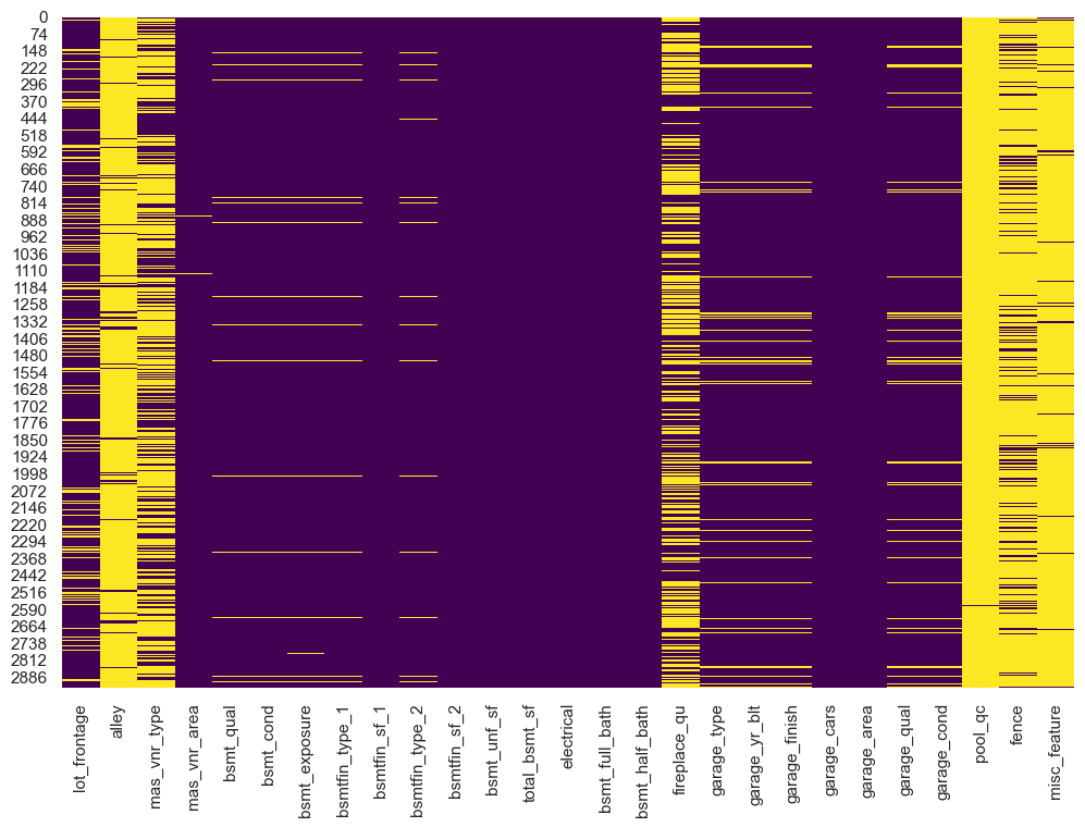
Sometimes visualizations help identify patterns in missing values. One thing I often do is print a heatmap of my dataframe to get a feel for where my missing values are. We’ll get into data visualization in future lessons but for now here is an example using the searborn library. We can see that several variables have a lot of missing values (alley, fireplace_qu, pool_qc, fence, misc_feature).
import seaborn as sns
sns.set(rc={'figure.figsize':(12, 8)})
ames_missing = ames[missing[missing].index]
sns.heatmap(ames_missing.isnull(), cmap='viridis', cbar=False);
Since we can’t drop all missing values in this data set (since it leaves us with no rows), we need to impute (“fill”) them in. There are several approaches we can use to do this; one of which uses the .fillna() method. This method has various options for filling, you can use a fixed value, the mean of the column, the previous non-nan value, etc:
import numpy as np

# example DataFrame with missing values
df = pd.DataFrame([[np.nan, 2, np.nan, 0],
                   [3, 4, np.nan, 1],
                   [np.nan, np.nan, np.nan, 5],
                   [np.nan, 3, np.nan, 4]],
                  columns=list('ABCD'))
df
| A | B | C | D | |
|---|---|---|---|---|
| 0 | NaN | 2.0 | NaN | 0 |
| 1 | 3.0 | 4.0 | NaN | 1 |
| 2 | NaN | NaN | NaN | 5 |
| 3 | NaN | 3.0 | NaN | 4 |
df.fillna(0) # fill with 0
| A | B | C | D | |
|---|---|---|---|---|
| 0 | 0.0 | 2.0 | 0.0 | 0 |
| 1 | 3.0 | 4.0 | 0.0 | 1 |
| 2 | 0.0 | 0.0 | 0.0 | 5 |
| 3 | 0.0 | 3.0 | 0.0 | 4 |
df.fillna(df.mean()) # fill with the mean
| A | B | C | D | |
|---|---|---|---|---|
| 0 | 3.0 | 2.0 | NaN | 0 |
| 1 | 3.0 | 4.0 | NaN | 1 |
| 2 | 3.0 | 3.0 | NaN | 5 |
| 3 | 3.0 | 3.0 | NaN | 4 |
df.bfill() # backward (upwards) fill from non-nan values
| A | B | C | D | |
|---|---|---|---|---|
| 0 | 3.0 | 2.0 | NaN | 0 |
| 1 | 3.0 | 4.0 | NaN | 1 |
| 2 | NaN | 3.0 | NaN | 5 |
| 3 | NaN | 3.0 | NaN | 4 |
df.ffill() # forward (downward) fill from non-nan values
| A | B | C | D | |
|---|---|---|---|---|
| 0 | NaN | 2.0 | NaN | 0 |
| 1 | 3.0 | 4.0 | NaN | 1 |
| 2 | 3.0 | 4.0 | NaN | 5 |
| 3 | 3.0 | 3.0 | NaN | 4 |
Applying custom functions#
There will be times when you want to apply a function that is not built-in to Pandas. For this, we have methods:
df.apply(), applies a function column-wise or row-wise across a dataframe (the function must be able to accept/return an array)df.applymap(), applies a function element-wise (for functions that accept/return single values at a time)series.apply()/series.map(), same as above but for Pandas series
For example, say you had the following custom function that defines if a home is considered a luxery home simply based on the price sold.
Note
Don’t worry, you’ll learn more about writing your own functions in future lessons!
def is_luxery_home(x):
    if x > 500000:
        return 'Luxery'
    else:
        return 'Non-luxery'

ames['saleprice'].apply(is_luxery_home)
0       Non-luxery
1       Non-luxery
2       Non-luxery
3       Non-luxery
4       Non-luxery
           ...
2925    Non-luxery
2926    Non-luxery
2927    Non-luxery
2928    Non-luxery
2929    Non-luxery
Name: saleprice, Length: 2930, dtype: object
This may have been better as a lambda function, which is just a shorter approach to writing functions. This may be a bit confusing but we’ll talk more about lambda functions in the writing functions lesson. For now, just think of it as being able to write a function for single use application on the fly.
ames['saleprice'].apply(lambda x: 'Luxery' if x > 500000 else 'Non-luxery')
0       Non-luxery
1       Non-luxery
2       Non-luxery
3       Non-luxery
4       Non-luxery
           ...
2925    Non-luxery
2926    Non-luxery
2927    Non-luxery
2928    Non-luxery
2929    Non-luxery
Name: saleprice, Length: 2930, dtype: object
You can even use functions that require additional arguments. Just specify the arguments in .apply():
def is_luxery_home(x, price):
    if x > price:
        return 'Luxery'
    else:
        return 'Non-luxery'

ames['saleprice'].apply(is_luxery_home, price=200000)
0           Luxery
1       Non-luxery
2       Non-luxery
3           Luxery
4       Non-luxery
           ...
2925    Non-luxery
2926    Non-luxery
2927    Non-luxery
2928    Non-luxery
2929    Non-luxery
Name: saleprice, Length: 2930, dtype: object
Sometimes we may have a function that we want to apply to every element across multiple columns. For example, say we wanted to convert several of the square footage variables to be represented as square meters. For this we can use the .applymap() method.
def convert_to_sq_meters(x):
    return x*0.092903

ames[['gr_liv_area', 'garage_area', 'lot_area']].map(convert_to_sq_meters)
| gr_liv_area | garage_area | lot_area | |
|---|---|---|---|
| 0 | 153.847368 | 49.052784 | 2946.883160 |
| 1 | 83.241088 | 67.819190 | 1075.073516 |
| 2 | 123.468087 | 28.985736 | 1320.801951 |
| 3 | 196.025330 | 48.495366 | 1032.152330 |
| 4 | 151.338987 | 44.779246 | 1280.203340 |
| ... | ... | ... | ... |
| 2925 | 93.181709 | 54.626964 | 732.725961 |
| 2926 | 83.798506 | 44.965052 | 820.798005 |
| 2927 | 90.115910 | 0.000000 | 965.355073 |
| 2928 | 129.042267 | 38.833454 | 925.313880 |
| 2929 | 185.806000 | 60.386950 | 889.732031 |
2930 rows × 3 columns
Exercises#
Questions:
Import the heart.csv dataset.
Are there any missing values in this data? If so, which columns? For these columns, fill the missing values with the value that appears most often (aka “mode”). This is a multi-step process and it would be worth reviewing the
.fillna()docs.Create a new column called
riskthat is equal to \( \frac{age}{\text{rest_bp} + chol + \text{max_hr}} \)Replace the values in the
rest_ecgcolumn so that:normal = normal
left ventricular hypertrophy = lvh
ST-T wave abnormality = stt_wav_abn
Computing environment#
Show code cell source
%load_ext watermark
%watermark -v -p jupyterlab,pandas,numpy,seaborn
Python implementation: CPython
Python version       : 3.12.4
IPython version      : 8.26.0

jupyterlab: 4.2.3
pandas    : 2.2.2
numpy     : 2.0.0
seaborn   : 0.13.2