Lesson 3c: Summarizing data#
What we have is a data glut.
- Vernor Vinge, Professor Emeritus of Mathematics, San Diego State University
Computing summary statistics across columns and various groupings within your dataset is a fundamental task in creating insights from your data. This lesson will focus on how we can compute various aggregations with Pandas Series and DataFrames.
Learning objectives#
By the end of this lesson you will be able to:
Compute summary statistics across an entire Series
Compute summary statistics across one or more columns in a DataFrame
Compute grouped-level summary statistics across one or more columns in a DataFrame
Simple aggregation#
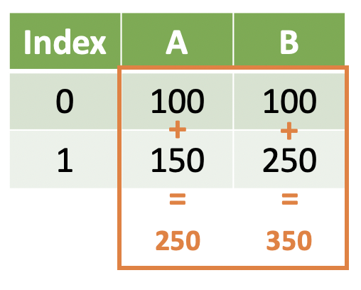
In the previous lesson we learned how to manipulate data across one or more variables within the row(s):
Note
We return the same number of elements that we started with. This is known as a window function, but you can also think of it as summarizing at the row-level.
We could achieve this result with the following code:
DataFrame['A'] + DataFrame['B']
We subset the two Series and then add them together using the + operator to achieve the sum. Note that we could also use some other operation on DataFrame['B'] as long as it returns the same number of elements.
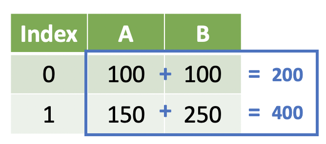
However, sometimes we want to work with data across rows within a variable – that is, aggregate/summarize values rowwise rather than columnwise.
Note
We return a single value representing some aggregation of the elements we started with. This is known as a summary function, but you can think of it as aggregating values across rows.
Summarizing a series#
The easiest way to summarize a specific series is by using bracket subsetting notation and the built-in Series methods (i.e. col.sum()):
import pandas as pd

ames = pd.read_csv('../data/ames_raw.csv')

ames['SalePrice'].sum()
np.int64(529732456)
Note that a single value was returned because this is a summary operation – we are summing the SalePrice variable across all rows.
There are other summary methods with a series:
ames['SalePrice'].mean()
np.float64(180796.0600682594)
ames['SalePrice'].median()
np.float64(160000.0)
ames['SalePrice'].std()
np.float64(79886.692356665)
All of the above methods work on quantitative variables but not character variables. However, there are summary methods that will work on all types of variables:
# Number of unique values in the neighborhood variable
ames['Neighborhood'].nunique()
28
# Most frequent value observed in the neighborhood variable
ames['Neighborhood'].mode()
0    NAmes
Name: Neighborhood, dtype: object
Knowledge check#
Questions:
What is the difference between a window operation and a summary operation?
What is the mean, median, and standard deviation of the above ground square footage (
Gr Liv Areavariable)?Find the count of each value observed in the
Neighborhoodcolumn. This may take a Google search. Would you consider the output a summary operation?
Video 🎥:
Describe method#
There is also a method describe() that provides a lot of this summary information – this is especially useful in initial exploratory data analysis.
ames['SalePrice'].describe()
count      2930.000000
mean     180796.060068
std       79886.692357
min       12789.000000
25%      129500.000000
50%      160000.000000
75%      213500.000000
max      755000.000000
Name: SalePrice, dtype: float64
Note
The describe() method will return different results depending on the type of the Series.
ames['Neighborhood'].describe()
count      2930
unique       28
top       NAmes
freq        443
Name: Neighborhood, dtype: object
Summarizing a DataFrame#
The above methods and operations are nice, but sometimes we want to work with multiple variables rather than just one. Recall how we select variables from a DataFrame:
Single-bracket subset notation
Pass a list of quoted variable names into the list
ames[['SalePrice', 'Gr Liv Area']]
We can use the same summary methods from the Series on the DataFrame to summarize data:
ames[['SalePrice', 'Gr Liv Area']].mean()
SalePrice      180796.060068
Gr Liv Area      1499.690444
dtype: float64
ames[['SalePrice', 'Gr Liv Area']].median()
SalePrice      160000.0
Gr Liv Area      1442.0
dtype: float64
This returns a pandas.core.series.Series object – the Index is the variable name and the values are the summarized values.
The Aggregation method#
While summary methods can be convenient, there are a few drawbacks to using them on DataFrames:
You can only apply one summary method at a time
You have to apply the same summary method to all variables
A Series is returned rather than a DataFrame – this makes it difficult to use the values in our analysis later
In order to get around these problems, the DataFrame has a powerful method .agg():
ames.agg({
    'SalePrice': ['mean']
})
| SalePrice | |
|---|---|
| mean | 180796.060068 |
There are a few things to notice about the agg() method:
A
dictis passed to the method with variable names as keys and a list of quoted summaries as valuesA DataFrame is returned with variable names as variables and summaries as rows
Tip
The .agg() method is just shorthand for .aggregate().
# I'm feeling quite verbose today!
ames.aggregate({
    'SalePrice': ['mean']
})
| SalePrice | |
|---|---|
| mean | 180796.060068 |
# I don't have that kind of time!
ames.agg({
    'SalePrice': ['mean']
})
| SalePrice | |
|---|---|
| mean | 180796.060068 |
We can extend this to multiple variables by adding elements to the dict:
ames.agg({
    'SalePrice': ['mean'],
    'Gr Liv Area': ['mean']
})
| SalePrice | Gr Liv Area | |
|---|---|---|
| mean | 180796.060068 | 1499.690444 |
And because the values of the dict are lists, we can do additional aggregations at the same time:
ames.agg({
    'SalePrice': ['mean', 'median'],
    'Gr Liv Area': ['mean', 'min']
})
| SalePrice | Gr Liv Area | |
|---|---|---|
| mean | 180796.060068 | 1499.690444 |
| median | 160000.000000 | NaN |
| min | NaN | 334.000000 |
Note
Not all variables have to have the same list of summaries. Note how NaN values fill in for those summary statistics not computed on a given variable.
Knowledge check#
Questions:
Fill in the blanks to compute the average number of rooms above ground (
TotRms AbvGrd) and the average number of bedrooms above ground (Bedroom AbvGr). What type of object is returned?ames[['______', '______']].______()
Use the
.agg()method to complete the same computation as above. How does the output differ?Fill in the blanks in the below code to calculate the minimum and maximum year built (
Year Built) and the mean and median number of garage stalls (Garage Cars):ames.agg({ '_____': ['min', '_____'], '_____': ['_____', 'median'] })
Video 🎥:
Describe method#
While agg() is a powerful method, the describe() method – similar to the Series describe() method – is a great choice during exploratory data analysis:
ames.describe()
| Order | PID | MS SubClass | Lot Frontage | Lot Area | Overall Qual | Overall Cond | Year Built | Year Remod/Add | Mas Vnr Area | ... | Wood Deck SF | Open Porch SF | Enclosed Porch | 3Ssn Porch | Screen Porch | Pool Area | Misc Val | Mo Sold | Yr Sold | SalePrice | |
|---|---|---|---|---|---|---|---|---|---|---|---|---|---|---|---|---|---|---|---|---|---|
| count | 2930.00000 | 2.930000e+03 | 2930.000000 | 2440.000000 | 2930.000000 | 2930.000000 | 2930.000000 | 2930.000000 | 2930.000000 | 2907.000000 | ... | 2930.000000 | 2930.000000 | 2930.000000 | 2930.000000 | 2930.000000 | 2930.000000 | 2930.000000 | 2930.000000 | 2930.000000 | 2930.000000 |
| mean | 1465.50000 | 7.144645e+08 | 57.387372 | 69.224590 | 10147.921843 | 6.094881 | 5.563140 | 1971.356314 | 1984.266553 | 101.896801 | ... | 93.751877 | 47.533447 | 23.011604 | 2.592491 | 16.002048 | 2.243345 | 50.635154 | 6.216041 | 2007.790444 | 180796.060068 |
| std | 845.96247 | 1.887308e+08 | 42.638025 | 23.365335 | 7880.017759 | 1.411026 | 1.111537 | 30.245361 | 20.860286 | 179.112611 | ... | 126.361562 | 67.483400 | 64.139059 | 25.141331 | 56.087370 | 35.597181 | 566.344288 | 2.714492 | 1.316613 | 79886.692357 |
| min | 1.00000 | 5.263011e+08 | 20.000000 | 21.000000 | 1300.000000 | 1.000000 | 1.000000 | 1872.000000 | 1950.000000 | 0.000000 | ... | 0.000000 | 0.000000 | 0.000000 | 0.000000 | 0.000000 | 0.000000 | 0.000000 | 1.000000 | 2006.000000 | 12789.000000 |
| 25% | 733.25000 | 5.284770e+08 | 20.000000 | 58.000000 | 7440.250000 | 5.000000 | 5.000000 | 1954.000000 | 1965.000000 | 0.000000 | ... | 0.000000 | 0.000000 | 0.000000 | 0.000000 | 0.000000 | 0.000000 | 0.000000 | 4.000000 | 2007.000000 | 129500.000000 |
| 50% | 1465.50000 | 5.354536e+08 | 50.000000 | 68.000000 | 9436.500000 | 6.000000 | 5.000000 | 1973.000000 | 1993.000000 | 0.000000 | ... | 0.000000 | 27.000000 | 0.000000 | 0.000000 | 0.000000 | 0.000000 | 0.000000 | 6.000000 | 2008.000000 | 160000.000000 |
| 75% | 2197.75000 | 9.071811e+08 | 70.000000 | 80.000000 | 11555.250000 | 7.000000 | 6.000000 | 2001.000000 | 2004.000000 | 164.000000 | ... | 168.000000 | 70.000000 | 0.000000 | 0.000000 | 0.000000 | 0.000000 | 0.000000 | 8.000000 | 2009.000000 | 213500.000000 |
| max | 2930.00000 | 1.007100e+09 | 190.000000 | 313.000000 | 215245.000000 | 10.000000 | 9.000000 | 2010.000000 | 2010.000000 | 1600.000000 | ... | 1424.000000 | 742.000000 | 1012.000000 | 508.000000 | 576.000000 | 800.000000 | 17000.000000 | 12.000000 | 2010.000000 | 755000.000000 |
8 rows × 39 columns
Warning
What is missing from the above result?
The string variables are missing! We can make describe() compute on all variable types using the include parameter and passing a list of data types to include:
ames.describe(include = ['int', 'float', 'object'])
| Order | PID | MS SubClass | MS Zoning | Lot Frontage | Lot Area | Street | Alley | Lot Shape | Land Contour | ... | Pool Area | Pool QC | Fence | Misc Feature | Misc Val | Mo Sold | Yr Sold | Sale Type | Sale Condition | SalePrice | |
|---|---|---|---|---|---|---|---|---|---|---|---|---|---|---|---|---|---|---|---|---|---|
| count | 2930.00000 | 2.930000e+03 | 2930.000000 | 2930 | 2440.000000 | 2930.000000 | 2930 | 198 | 2930 | 2930 | ... | 2930.000000 | 13 | 572 | 106 | 2930.000000 | 2930.000000 | 2930.000000 | 2930 | 2930 | 2930.000000 |
| unique | NaN | NaN | NaN | 7 | NaN | NaN | 2 | 2 | 4 | 4 | ... | NaN | 4 | 4 | 5 | NaN | NaN | NaN | 10 | 6 | NaN |
| top | NaN | NaN | NaN | RL | NaN | NaN | Pave | Grvl | Reg | Lvl | ... | NaN | Ex | MnPrv | Shed | NaN | NaN | NaN | WD | Normal | NaN |
| freq | NaN | NaN | NaN | 2273 | NaN | NaN | 2918 | 120 | 1859 | 2633 | ... | NaN | 4 | 330 | 95 | NaN | NaN | NaN | 2536 | 2413 | NaN |
| mean | 1465.50000 | 7.144645e+08 | 57.387372 | NaN | 69.224590 | 10147.921843 | NaN | NaN | NaN | NaN | ... | 2.243345 | NaN | NaN | NaN | 50.635154 | 6.216041 | 2007.790444 | NaN | NaN | 180796.060068 |
| std | 845.96247 | 1.887308e+08 | 42.638025 | NaN | 23.365335 | 7880.017759 | NaN | NaN | NaN | NaN | ... | 35.597181 | NaN | NaN | NaN | 566.344288 | 2.714492 | 1.316613 | NaN | NaN | 79886.692357 |
| min | 1.00000 | 5.263011e+08 | 20.000000 | NaN | 21.000000 | 1300.000000 | NaN | NaN | NaN | NaN | ... | 0.000000 | NaN | NaN | NaN | 0.000000 | 1.000000 | 2006.000000 | NaN | NaN | 12789.000000 |
| 25% | 733.25000 | 5.284770e+08 | 20.000000 | NaN | 58.000000 | 7440.250000 | NaN | NaN | NaN | NaN | ... | 0.000000 | NaN | NaN | NaN | 0.000000 | 4.000000 | 2007.000000 | NaN | NaN | 129500.000000 |
| 50% | 1465.50000 | 5.354536e+08 | 50.000000 | NaN | 68.000000 | 9436.500000 | NaN | NaN | NaN | NaN | ... | 0.000000 | NaN | NaN | NaN | 0.000000 | 6.000000 | 2008.000000 | NaN | NaN | 160000.000000 |
| 75% | 2197.75000 | 9.071811e+08 | 70.000000 | NaN | 80.000000 | 11555.250000 | NaN | NaN | NaN | NaN | ... | 0.000000 | NaN | NaN | NaN | 0.000000 | 8.000000 | 2009.000000 | NaN | NaN | 213500.000000 |
| max | 2930.00000 | 1.007100e+09 | 190.000000 | NaN | 313.000000 | 215245.000000 | NaN | NaN | NaN | NaN | ... | 800.000000 | NaN | NaN | NaN | 17000.000000 | 12.000000 | 2010.000000 | NaN | NaN | 755000.000000 |
11 rows × 82 columns
Grouped aggregation#
In the section above, we talked about summary operations in the context of collapsing a DataFrame to a single row. This is not always the case – often we are interested in examining specific groups in our data and we want to perform summary operations for these groups. Thus, we are interested in collapsing to a single row per group. This is known as a grouped aggregation.
For example, in the following illustration we are interested in finding the sum of variable B for each category/value in variable A.

This can be useful when we want to aggregate by category:
Maximum temperature by month
Total home runs by team
Total sales by neighborhood
Average number of seats by plane manufacturer
When we summarize by groups, we can use the same aggregation methods we previously did
Summary methods for a specific summary operation:
DataFrame.sum()Describe method for a collection of summary operations:
DataFrame.describe()Agg method for flexibility in summary operations:
DataFrame.agg({'VariableName': ['sum', 'mean']})
The only difference is the need to set the DataFrame group prior to aggregating. We can set the DataFrame group by calling the DataFrame.groupby() method and passing a variable name:
ames_grp = ames.groupby('Neighborhood')
ames_grp
<pandas.core.groupby.generic.DataFrameGroupBy object at 0x108c694f0>
Notice that a DataFrame doesn’t print when it’s grouped. The groupby() method is just setting the group - you can see the changed DataFrame class:
type(ames_grp)
pandas.core.groupby.generic.DataFrameGroupBy
The groupby object is really just a dictionary of index-mappings, which we could look at if we wanted to:
ames_grp.groups
{'Blmngtn': [52, 53, 468, 469, 470, 471, 472, 473, 1080, 1081, 1082, 1083, 1084, 1741, 1742, 1743, 1744, 2419, 2420, 2421, 2422, 2423, 2424, 2425, 2426, 2427, 2428, 2429], 'Blueste': [298, 299, 932, 933, 934, 935, 1542, 1543, 2225, 2227], 'BrDale': [29, 30, 31, 402, 403, 404, 405, 406, 407, 1039, 1040, 1041, 1042, 1043, 1044, 1045, 1675, 1676, 1677, 1678, 1679, 2364, 2365, 2366, 2367, 2368, 2369, 2370, 2371, 2372], 'BrkSide': [129, 130, 191, 192, 193, 194, 195, 196, 197, 198, 199, 614, 615, 728, 729, 730, 731, 732, 733, 734, 735, 736, 737, 738, 739, 740, 741, 742, 743, 744, 745, 746, 747, 748, 1219, 1220, 1221, 1222, 1327, 1328, 1329, 1330, 1331, 1332, 1333, 1334, 1335, 1336, 1337, 1338, 1339, 1340, 1341, 1342, 1343, 1344, 1345, 1348, 1349, 1350, 1351, 1352, 1353, 1354, 1355, 1901, 1902, 1903, 1904, 2005, 2006, 2007, 2008, 2009, 2010, 2011, 2012, 2013, 2014, 2015, 2016, 2017, 2018, 2019, 2020, 2022, 2023, 2024, 2025, 2554, 2555, 2556, 2557, 2670, 2671, 2672, 2673, 2675, 2676, 2677, ...], 'ClearCr': [208, 209, 210, 228, 229, 232, 233, 255, 779, 781, 782, 785, 833, 834, 1374, 1392, 1395, 1398, 1399, 1400, 1401, 1402, 1406, 1429, 1430, 2045, 2071, 2072, 2073, 2077, 2115, 2116, 2117, 2118, 2701, 2725, 2726, 2727, 2730, 2731, 2764, 2765, 2766, 2767], 'CollgCr': [249, 250, 251, 252, 256, 257, 258, 259, 260, 261, 262, 263, 264, 265, 266, 267, 268, 269, 270, 271, 272, 818, 819, 820, 821, 822, 823, 824, 825, 826, 827, 828, 829, 830, 831, 835, 836, 837, 838, 839, 840, 841, 842, 843, 844, 845, 846, 847, 848, 849, 850, 851, 852, 853, 854, 855, 856, 857, 858, 859, 860, 861, 862, 863, 864, 865, 866, 867, 868, 869, 870, 871, 872, 873, 874, 875, 876, 877, 878, 879, 880, 881, 882, 883, 1423, 1424, 1425, 1426, 1431, 1432, 1433, 1434, 1435, 1436, 1437, 1438, 1439, 1440, 1441, 1442, ...], 'Crawfor': [293, 294, 295, 296, 297, 300, 308, 912, 915, 917, 918, 919, 920, 921, 922, 923, 924, 925, 926, 927, 928, 929, 930, 931, 936, 937, 938, 944, 1523, 1524, 1525, 1526, 1528, 1530, 1531, 1532, 1533, 1534, 1535, 1536, 1537, 1538, 1539, 1540, 1541, 1559, 1560, 1561, 1562, 2196, 2197, 2198, 2199, 2201, 2202, 2203, 2204, 2205, 2206, 2207, 2208, 2209, 2210, 2211, 2212, 2213, 2214, 2215, 2216, 2217, 2218, 2219, 2220, 2221, 2222, 2223, 2224, 2226, 2228, 2229, 2230, 2245, 2246, 2850, 2853, 2854, 2857, 2858, 2859, 2860, 2861, 2862, 2863, 2864, 2865, 2866, 2867, 2868, 2869, 2870, ...], 'Edwards': [234, 235, 236, 237, 238, 239, 240, 241, 242, 243, 273, 274, 275, 276, 277, 278, 279, 280, 281, 282, 283, 284, 287, 762, 763, 764, 765, 766, 767, 783, 784, 786, 787, 788, 789, 790, 791, 792, 793, 794, 795, 796, 797, 798, 884, 885, 886, 887, 888, 889, 890, 891, 892, 893, 894, 895, 896, 897, 898, 899, 900, 901, 902, 903, 904, 1375, 1403, 1404, 1405, 1407, 1408, 1409, 1410, 1411, 1412, 1413, 1414, 1415, 1416, 1417, 1485, 1486, 1487, 1488, 1489, 1490, 1491, 1492, 1493, 1494, 1495, 1496, 1497, 1498, 1499, 1500, 1501, 1502, 1503, 1504, ...], 'Gilbert': [4, 5, 9, 10, 11, 12, 13, 16, 18, 51, 54, 55, 56, 57, 58, 344, 345, 346, 347, 348, 353, 354, 355, 356, 357, 358, 359, 360, 361, 362, 363, 364, 369, 464, 465, 466, 467, 474, 475, 476, 477, 478, 479, 480, 481, 483, 484, 485, 486, 487, 488, 489, 490, 491, 492, 493, 992, 993, 994, 995, 996, 997, 998, 1003, 1004, 1005, 1006, 1007, 1013, 1015, 1085, 1086, 1087, 1088, 1089, 1090, 1092, 1093, 1094, 1095, 1096, 1097, 1615, 1616, 1617, 1618, 1619, 1621, 1622, 1623, 1624, 1625, 1626, 1627, 1628, 1629, 1630, 1638, 1727, 1728, ...], 'Greens': [106, 107, 575, 1857, 2518, 2519, 2520, 2521], 'GrnHill': [2256, 2892], 'IDOTRR': [205, 206, 301, 302, 303, 304, 305, 306, 307, 726, 727, 754, 755, 758, 759, 760, 939, 940, 941, 942, 943, 945, 1359, 1360, 1361, 1362, 1363, 1364, 1365, 1368, 1369, 1370, 1544, 1545, 1546, 1547, 1548, 1549, 1550, 1551, 1552, 1553, 1554, 1555, 1556, 1557, 1558, 1610, 2030, 2031, 2032, 2033, 2034, 2035, 2036, 2037, 2038, 2039, 2043, 2231, 2232, 2233, 2234, 2235, 2236, 2237, 2238, 2239, 2240, 2241, 2242, 2243, 2244, 2669, 2690, 2691, 2692, 2693, 2694, 2695, 2696, 2697, 2872, 2873, 2874, 2875, 2876, 2877, 2878, 2879, 2880, 2881, 2882], 'Landmrk': [2788], 'MeadowV': [326, 327, 328, 329, 330, 331, 332, 973, 975, 977, 978, 979, 1593, 1594, 1595, 1596, 1597, 1599, 1600, 2283, 2284, 2285, 2286, 2287, 2288, 2289, 2290, 2908, 2909, 2910, 2913, 2914, 2916, 2917, 2918, 2919, 2920], 'Mitchel': [309, 310, 311, 312, 313, 322, 323, 324, 325, 333, 334, 335, 336, 337, 338, 339, 340, 946, 947, 948, 949, 950, 951, 952, 953, 954, 969, 970, 971, 972, 974, 976, 980, 981, 982, 983, 984, 985, 986, 987, 988, 1563, 1564, 1565, 1566, 1567, 1568, 1569, 1588, 1589, 1590, 1591, 1592, 1598, 1601, 1602, 1603, 1604, 1605, 1606, 1607, 1608, 1609, 2247, 2248, 2249, 2250, 2251, 2252, 2253, 2254, 2277, 2278, 2279, 2280, 2281, 2282, 2291, 2292, 2293, 2294, 2295, 2296, 2297, 2298, 2299, 2300, 2301, 2302, 2303, 2304, 2885, 2886, 2887, 2888, 2889, 2890, 2903, 2904, 2905, ...], 'NAmes': [0, 1, 2, 3, 23, 24, 25, 26, 27, 28, 117, 119, 120, 121, 122, 123, 124, 125, 126, 127, 128, 131, 132, 133, 134, 135, 136, 137, 138, 139, 140, 141, 142, 143, 144, 145, 146, 147, 148, 149, 150, 151, 152, 153, 154, 155, 156, 157, 159, 160, 161, 162, 163, 164, 165, 166, 167, 168, 341, 342, 343, 392, 393, 394, 395, 396, 397, 398, 399, 400, 401, 418, 419, 593, 594, 595, 599, 600, 601, 602, 603, 604, 605, 606, 607, 608, 609, 610, 611, 612, 613, 616, 617, 618, 619, 620, 621, 622, 623, 624, ...], 'NPkVill': [32, 33, 34, 35, 408, 409, 410, 411, 412, 413, 414, 415, 416, 417, 1046, 1047, 1048, 1680, 1681, 1682, 2373, 2376, 2377], 'NWAmes': [19, 20, 21, 110, 111, 112, 113, 114, 115, 116, 118, 370, 371, 372, 373, 374, 375, 376, 377, 378, 379, 380, 381, 382, 387, 388, 389, 390, 391, 579, 580, 581, 582, 583, 584, 585, 586, 587, 588, 589, 590, 591, 592, 596, 597, 598, 1016, 1017, 1018, 1019, 1020, 1021, 1022, 1023, 1024, 1025, 1026, 1027, 1028, 1029, 1030, 1031, 1032, 1185, 1186, 1187, 1188, 1189, 1190, 1191, 1197, 1198, 1199, 1200, 1201, 1203, 1643, 1644, 1645, 1646, 1647, 1648, 1649, 1650, 1651, 1652, 1653, 1654, 1655, 1656, 1657, 1658, 1659, 1660, 1661, 1863, 1864, 1865, 1866, 1867, ...], 'NoRidge': [59, 60, 61, 62, 63, 64, 65, 90, 91, 92, 494, 495, 496, 497, 498, 499, 500, 501, 502, 503, 504, 505, 564, 1098, 1099, 1100, 1101, 1102, 1103, 1104, 1105, 1106, 1107, 1108, 1109, 1157, 1158, 1760, 1761, 1762, 1763, 1764, 1765, 1766, 1767, 1768, 1769, 1770, 1771, 1772, 1773, 1774, 1832, 1833, 2442, 2443, 2444, 2445, 2446, 2447, 2448, 2449, 2450, 2451, 2452, 2453, 2499, 2500, 2501, 2502, 2503], 'NridgHt': [36, 37, 38, 39, 40, 41, 42, 43, 44, 45, 46, 47, 48, 49, 50, 420, 421, 422, 423, 424, 425, 426, 427, 428, 429, 430, 431, 432, 433, 434, 435, 436, 437, 438, 439, 440, 441, 442, 443, 444, 445, 446, 447, 448, 449, 450, 451, 452, 453, 454, 455, 456, 457, 458, 459, 460, 461, 462, 463, 482, 1050, 1051, 1052, 1053, 1054, 1055, 1056, 1057, 1058, 1059, 1060, 1061, 1062, 1063, 1064, 1065, 1066, 1067, 1068, 1069, 1070, 1071, 1072, 1073, 1074, 1075, 1076, 1077, 1078, 1079, 1091, 1684, 1685, 1686, 1687, 1688, 1689, 1690, 1691, 1692, ...], 'OldTown': [158, 169, 170, 171, 172, 173, 174, 175, 176, 177, 178, 179, 180, 181, 182, 183, 184, 185, 186, 187, 188, 189, 190, 200, 201, 202, 203, 204, 207, 650, 654, 655, 656, 657, 658, 659, 660, 661, 662, 663, 664, 665, 691, 692, 693, 694, 695, 696, 697, 698, 699, 700, 701, 702, 703, 704, 705, 706, 707, 708, 709, 710, 711, 712, 713, 714, 715, 716, 717, 718, 719, 720, 721, 722, 723, 724, 725, 749, 750, 751, 752, 753, 756, 757, 1254, 1255, 1257, 1258, 1259, 1283, 1284, 1285, 1286, 1287, 1288, 1289, 1290, 1291, 1292, 1293, ...], 'SWISU': [211, 212, 213, 214, 285, 286, 288, 289, 290, 291, 292, 905, 906, 907, 908, 909, 910, 911, 913, 914, 916, 1515, 1516, 1517, 1518, 1519, 1520, 1521, 1522, 1527, 1529, 2047, 2080, 2194, 2195, 2200, 2703, 2704, 2842, 2845, 2846, 2847, 2848, 2849, 2851, 2852, 2855, 2856], 'Sawyer': [83, 84, 85, 86, 87, 88, 89, 108, 215, 216, 217, 218, 219, 220, 221, 222, 223, 224, 225, 226, 227, 230, 231, 554, 555, 556, 557, 558, 559, 560, 561, 562, 578, 761, 768, 769, 770, 771, 772, 773, 774, 775, 776, 777, 778, 780, 1149, 1150, 1151, 1152, 1153, 1154, 1156, 1371, 1372, 1373, 1376, 1377, 1378, 1379, 1380, 1381, 1382, 1383, 1384, 1385, 1386, 1387, 1388, 1389, 1390, 1391, 1393, 1394, 1396, 1397, 1818, 1819, 1820, 1821, 1822, 1823, 1824, 1825, 1826, 1829, 1830, 1831, 1861, 2044, 2048, 2049, 2050, 2051, 2052, 2053, 2054, 2055, 2056, 2057, ...], 'SawyerW': [72, 73, 74, 75, 76, 77, 78, 79, 80, 81, 82, 244, 245, 246, 247, 248, 253, 254, 533, 534, 535, 536, 537, 538, 539, 540, 541, 542, 543, 544, 545, 546, 547, 548, 549, 550, 551, 552, 553, 799, 800, 801, 802, 803, 804, 805, 806, 807, 808, 809, 810, 811, 812, 813, 814, 815, 816, 817, 832, 1131, 1132, 1133, 1134, 1135, 1136, 1137, 1138, 1139, 1140, 1141, 1142, 1143, 1144, 1145, 1146, 1147, 1148, 1418, 1419, 1420, 1421, 1422, 1427, 1428, 1806, 1807, 1808, 1809, 1810, 1811, 1812, 1813, 1814, 1815, 1816, 1817, 2089, 2090, 2091, 2092, ...], 'Somerst': [22, 66, 67, 68, 69, 70, 71, 93, 94, 95, 96, 97, 98, 99, 100, 101, 102, 103, 104, 105, 109, 383, 384, 385, 386, 506, 507, 508, 509, 510, 511, 512, 513, 514, 515, 516, 517, 518, 519, 520, 521, 522, 523, 524, 525, 526, 527, 528, 529, 530, 531, 532, 565, 566, 567, 568, 569, 570, 571, 572, 573, 1110, 1111, 1112, 1113, 1114, 1115, 1116, 1117, 1118, 1119, 1120, 1121, 1122, 1123, 1124, 1125, 1126, 1127, 1128, 1129, 1130, 1159, 1160, 1161, 1162, 1163, 1164, 1165, 1166, 1167, 1168, 1169, 1170, 1171, 1172, 1173, 1174, 1175, 1176, ...], 'StoneBr': [6, 7, 8, 14, 15, 17, 349, 350, 351, 352, 365, 366, 367, 368, 999, 1000, 1001, 1002, 1008, 1009, 1010, 1011, 1012, 1014, 1620, 1631, 1632, 1633, 1634, 1635, 1636, 1637, 1639, 1640, 1641, 1642, 2322, 2326, 2327, 2328, 2329, 2330, 2331, 2332, 2333, 2334, 2335, 2336, 2339, 2340, 2341], 'Timber': [314, 315, 316, 317, 318, 319, 320, 321, 955, 956, 957, 958, 959, 960, 961, 962, 963, 964, 965, 966, 967, 968, 1570, 1571, 1572, 1573, 1574, 1575, 1576, 1577, 1578, 1579, 1580, 1581, 1582, 1583, 1584, 1585, 1586, 1587, 2255, 2257, 2258, 2259, 2260, 2261, 2262, 2263, 2264, 2265, 2266, 2267, 2268, 2269, 2270, 2271, 2272, 2273, 2274, 2275, 2276, 2891, 2893, 2894, 2895, 2896, 2897, 2898, 2899, 2900, 2901, 2902], 'Veenker': [563, 574, 576, 577, 1155, 1178, 1179, 1180, 1181, 1182, 1183, 1827, 1828, 1853, 1854, 1855, 1856, 1858, 1859, 1860, 2498, 2516, 2517, 2522]}
We can also access a group using the .get_group() method:
# get the Bloomington neighborhood group
ames_grp.get_group('Blmngtn').head()
| Order | PID | MS SubClass | MS Zoning | Lot Frontage | Lot Area | Street | Alley | Lot Shape | Land Contour | ... | Pool Area | Pool QC | Fence | Misc Feature | Misc Val | Mo Sold | Yr Sold | Sale Type | Sale Condition | SalePrice | |
|---|---|---|---|---|---|---|---|---|---|---|---|---|---|---|---|---|---|---|---|---|---|
| 52 | 53 | 528228285 | 120 | RL | 43.0 | 3203 | Pave | NaN | Reg | Lvl | ... | 0 | NaN | NaN | NaN | 0 | 1 | 2010 | WD | Normal | 160000 |
| 53 | 54 | 528228440 | 120 | RL | 43.0 | 3182 | Pave | NaN | Reg | Lvl | ... | 0 | NaN | NaN | NaN | 0 | 4 | 2010 | WD | Normal | 192000 |
| 468 | 469 | 528228290 | 120 | RL | 53.0 | 3684 | Pave | NaN | Reg | Lvl | ... | 0 | NaN | NaN | NaN | 0 | 6 | 2009 | WD | Normal | 174000 |
| 469 | 470 | 528228295 | 120 | RL | 51.0 | 3635 | Pave | NaN | Reg | Lvl | ... | 0 | NaN | NaN | NaN | 0 | 5 | 2009 | WD | Normal | 175900 |
| 470 | 471 | 528228435 | 120 | RL | 43.0 | 3182 | Pave | NaN | Reg | Lvl | ... | 0 | NaN | NaN | NaN | 0 | 5 | 2009 | WD | Normal | 192500 |
5 rows × 82 columns
If we then call an aggregation method after our groupby() call, we will see the DataFrame returned with group-level aggregations:
ames.groupby('Neighborhood').agg({'SalePrice': ['mean', 'median']}).head()
| SalePrice | ||
|---|---|---|
| mean | median | |
| Neighborhood | ||
| Blmngtn | 196661.678571 | 191500.0 |
| Blueste | 143590.000000 | 130500.0 |
| BrDale | 105608.333333 | 106000.0 |
| BrkSide | 124756.250000 | 126750.0 |
| ClearCr | 208662.090909 | 197500.0 |
This process always follows this model:

Groups as index vs. variables#
Note
Notice that the grouped variable becomes the Index in our example!
ames.groupby('Neighborhood').agg({'SalePrice': ['mean', 'median']}).index
Index(['Blmngtn', 'Blueste', 'BrDale', 'BrkSide', 'ClearCr', 'CollgCr',
       'Crawfor', 'Edwards', 'Gilbert', 'Greens', 'GrnHill', 'IDOTRR',
       'Landmrk', 'MeadowV', 'Mitchel', 'NAmes', 'NPkVill', 'NWAmes',
       'NoRidge', 'NridgHt', 'OldTown', 'SWISU', 'Sawyer', 'SawyerW',
       'Somerst', 'StoneBr', 'Timber', 'Veenker'],
      dtype='object', name='Neighborhood')
This is the default behavior of pandas, and probably how pandas wants to be used. In fact, this is the fastest way to do it, but it’s a matter of less than a millisecond. However, you aren’t always going to see people group by the index. Instead of setting the group as the index, we can set the group as a variable.
Tip
The grouped variable can remain a Series/variable by adding the as_index = False parameter/argument to groupby().
ames.groupby('Neighborhood', as_index=False).agg({'SalePrice': ['mean', 'median']}).head()
| Neighborhood | SalePrice | ||
|---|---|---|---|
| mean | median | ||
| 0 | Blmngtn | 196661.678571 | 191500.0 |
| 1 | Blueste | 143590.000000 | 130500.0 |
| 2 | BrDale | 105608.333333 | 106000.0 |
| 3 | BrkSide | 124756.250000 | 126750.0 |
| 4 | ClearCr | 208662.090909 | 197500.0 |
Grouping by multiple variables#
Sometimes we have multiple categories by which we’d like to group. To extend our example, assume we want to find the average sale price by neighborhood AND year sold. We can pass a list of variable names to the groupby() method:
ames.groupby(['Neighborhood', 'Yr Sold'], as_index=False).agg({'SalePrice': 'mean'})
| Neighborhood | Yr Sold | SalePrice | |
|---|---|---|---|
| 0 | Blmngtn | 2006 | 214424.454545 |
| 1 | Blmngtn | 2007 | 194671.500000 |
| 2 | Blmngtn | 2008 | 190714.400000 |
| 3 | Blmngtn | 2009 | 177266.666667 |
| 4 | Blmngtn | 2010 | 176000.000000 |
| ... | ... | ... | ... |
| 125 | Timber | 2010 | 224947.625000 |
| 126 | Veenker | 2006 | 270000.000000 |
| 127 | Veenker | 2007 | 253577.777778 |
| 128 | Veenker | 2008 | 225928.571429 |
| 129 | Veenker | 2009 | 253962.500000 |
130 rows × 3 columns
Knowledge check#
Questions:
How would you convert the following statement into a grouped aggregation syntax: “what is the average above ground square footage of homes based on neighbhorhood and bedroom count”?
Compute the above statement (variable hints:
Gr Liv Area= above ground square footage,Neighborhood= neighborhood,Bedroom AbvGr= bedroom count).Using the results from #2, find out which neighborhoods have 1 bedrooms homes that average more than 1500 above ground square feet.
Video 🎥:
Exercises#
Questions:
Using the Ames housing data…
What neighbhorhood has the largest median sales price? (hint: check out
sort_values())What is the mean and median sales price based on the number of bedrooms (
Bedroom AbvGr)?Which neighbhorhood has the largest median sales price for 3 bedroom homes? Which neighborhood has the smallest median sales price for 3 bedroom homes?
Compute the sales price per square footage (
Gr Liv Area) per home. Call this variableprice_per_sqft. Now compute the medianprice_per_sqftper neighborhood. Which neighborhood has the largest medianprice_per_sqft? Does this differ from the neighborhood identified in #1? What information does this provide you?
Computing environment#
Show code cell source
%load_ext watermark
%watermark -v -p jupyterlab,pandas
Python implementation: CPython
Python version       : 3.12.4
IPython version      : 8.26.0

jupyterlab: 4.2.3
pandas    : 2.2.2