2 Lesson 1a: R & RStudio
This lesson is designed to help you get up and running with R and RStudio. It will also provide you with some tips for getting help as you start writing R code and differentiating errors, warnings, and messages (because we will experience these daily!).
2.1 Learning objectives
Upon completing this module you will:
- Understand the difference between R and RStudio.
- Have R and RStudio installed on your computer.
- Be able to navigate the RStudio IDE.
- Know how to get help as you first start learning R.
- Differentiate errors, warnings, and messages.
- Know what additional resources are available to go deeper.
2.2 R vs. RStudio
When students first learn about R and RStudio, they are often confused on how the two differentiate. R is a programming language that runs computations, while RStudio is an integrated development environment (IDE) that provides an interface by adding many convenient features and tools. An analogy used by Ismay and Kim (2019) helps put this into perspective. “R is like a car’s engine while RStudio is like a car’s dashboard…just as the way of having access to a speedometer, rearview mirrors, and a navigation system makes driving much easier, using RStudio’s interface makes using R much easier as well.”
![Analogy of difference between R and RStudio [@ismay2019statistical]](images/R_vs_RStudio_1.png)
Figure 2.1: Analogy of difference between R and RStudio (Ismay and Kim 2019)
It is important to note that one can write R and do nearly everything you are going to do in this course without using RStudio. However, RStudio has lots of features that make writing, executing, and organizing your R code so much easier. Moreover, realize that there are other IDEs and platforms that you can use (i.e. VS code, Radiant, jupyter) to write and execute R code; however, RStudio has become the defacto IDE for R and is heavily used throughout the R community.
Since RStudio has lots of features, it takes time to learn them. A good resource to learn more about RStudio are the R Studio Essentials collection of videos.
2.3 Installing R and RStudio
It is important that you install R first and then install RStudio. You can download and install R from CRAN, the Comprehensive R Archive Network. It is highly recommended to install a precompiled binary distribution for your operating system (OS); follow these instructions:
- Go to https://cloud.r-project.org/
- Select the installer for your operating system:
- If you are a Windows user: Click on “Download R for Windows”, then click on “base”, then click on the Download link.
- If you are macOS user: Click on “Download R for (Mac) OS X”, then under “Latest release:” click on R-X.X.X.pkg, where R-X.X.X is the version number. For example, the latest version of R as of April 25, 2022 was R-4.2.0.
- If you are a Linux user: Click on “Download R for Linux” and choose your distribution for more information on installing R for your setup.
- Follow the instructions of the installer.
Next, you can download RStudio’s IDE by following these instructions:
- Go to RStudio for desktop https://www.rstudio.com/products/rstudio/download/
- Scroll down to “Installers for Supported Platforms” near the bottom of the page.
- Select the install file for your OS.
- Follow the instructions of the installer.
Installing R and RStudio should be fairly straightforward. However, a great set of detailed step-by-step instructions is in Rafael Irizarry’s Introduction to Data Science book (Irizarry 2019).
After you install R and RStudio on your computer, you’ll have two new programs (also called applications) you can open. The R application icon looks like the left image below while the RStudio icon looks like the right image. We’ll always work in RStudio and not in the R application so be sure to select the correct icon.
Figure 2.2: Use the RStudio icon (right) and not the R icon (left) to launch your R project. (Ismay and Kim 2019)
If your OS allows, pin the RStudio icon to your desktop or Dock and keep the R icon in another location (i.e. Applications for Mac users). This makes it natural and efficient to always go to the RStudio icon on your desktop for launching the program.
After you open RStudio, you should see something similar to the following image. Note that slight differences might exist depending on the version of your RStudio interface.
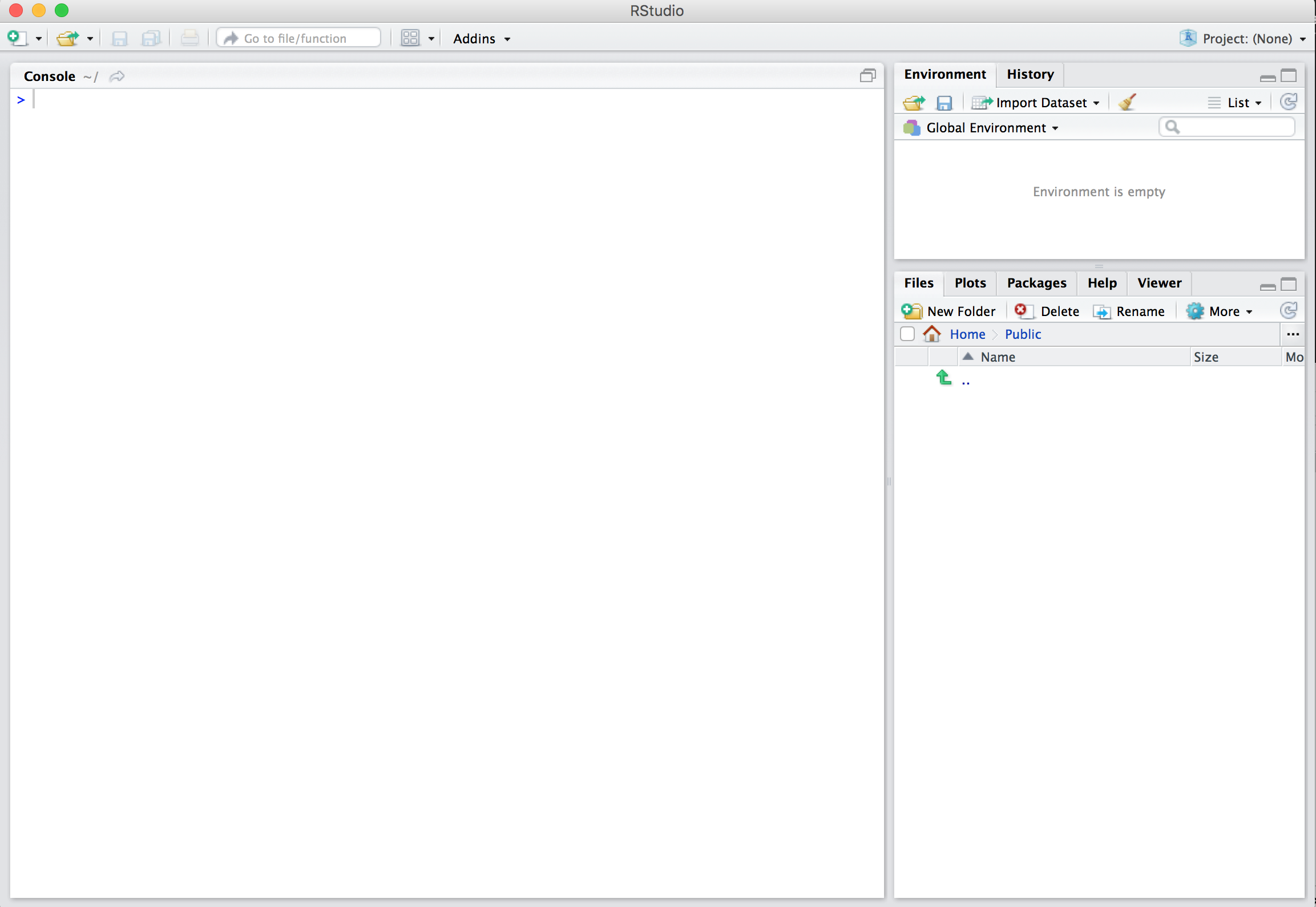
Figure 2.3: RStudio interface to R.
You are now ready to start programming!
2.4 Understanding the RStudio IDE
The RStudio IDE is where all the action happens. There are four fundamental windows in the IDE, each with their own purpose. I discuss each briefly below but I highly suggest Oscar Torres-Reyna’s Introduction to RStudio for a thorough understanding of the console1.
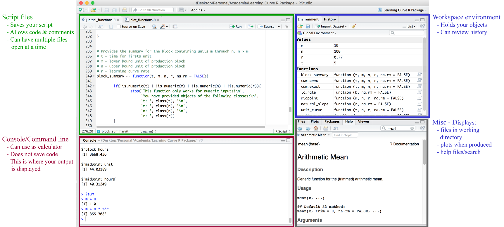
Figure 2.4: The four fundamental windows within the RStudio IDE
2.4.1 Script Editor
The top left window is where your script files will display. There are multiple forms of script files but the basic one to start with is the .R file. To create a new file you use the File » New File menu. To open an existing file you use either the File » Open File… menu or the Recent Files menu to select from recently opened files. RStudio’s source editor includes a variety of productivity enhancing features including syntax highlighting, code completion, multiple-file editing, and find/replace. A good introduction to the script editor was written by RStudio’s Josh Paulson2.
The script editor is a great place to put code you care about. Keep experimenting in the console, but once you have written code that works and does what you want, put it in the script editor. RStudio will automatically save the contents of the editor when you quit RStudio, and will automatically load it when you re-open. Nevertheless, it’s a good idea to save your scripts regularly and to back them up.
To execute the code in the script editor you have two options:
- Place the cursor on the line that you would like to execute and execute Cmd/Ctrl + Enter. Alternatively, you could hit the Run button in the toolbar.
- If you want to run all lines of code in the script then you can highlight the lines you want to run and then execute one of the options in #1.
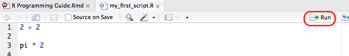
Figure 2.5: Execute lines of code in your script with Cmd/Ctrl + Enter or using the Run button.
2.4.2 Workspace Environment
The top right window is the workspace environment which captures much of your current R working environment and includes any user-defined objects (vectors, matrices, data frames, lists, functions). When saving your R working session, these are the components along with the script files that will be saved in your working directory, which is the default location for all file inputs and outputs. To get or set your working directory so you can direct where your files are saved:
# returns path for the current working directory
getwd()

# set the working directory to a specified directory
setwd("path/of/directory")
For example, if I call getwd() the file path “/Users/b294776/Desktop” is returned. If I want to set the working directory to the “Workspace” folder within the “Desktop” directory I would use setwd("/Users/b294776/Desktop/Workspace"). Now if I call getwd() again it returns “/Users/b294776/Desktop/Workspace”. An alternative solution is to go to the following location in your toolbar Session » Set Working Directory » Choose Directory and select the directory of choice (much easier!).
The workspace environment will also list your user defined objects such as vectors, matrices, data frames, lists, and functions. For example, if you type the following in your console:
You will now see x and y listed in your workspace environment. To identify or remove the objects (i.e. vectors, data frames, user defined functions, etc.) in your current R environment:
# list all objects
ls()

# identify if an R object with a given name is present
exists("x")

# remove defined object from the environment
rm(x)

# you can remove multiple objects
rm(x, y)

# basically removes everything in the working environment -- use with caution!
rm(list = ls())
If you have a lot of objects in your workspace environment you can use the 🧹 icon in the workspace environment tab to clear out everything.
You can also view previous commands in the workspace environment by clicking the History tab, by simply pressing the up arrow on your keyboard, or by typing into the console:
2.4.3 Console
The bottom left window contains the console. You can code directly in this window but it will not save your code. It is best to use this window when you are simply wanting to perform calculator type functions. This is also where your outputs will be presented when you run code in your script. Go ahead and type the following in your console:
2.4.4 Misc. Displays
The bottom right window contains multiple tabs. The Files tab allows you to see which files are available in your working directory. The Plots tab will display any plots/graphics that are produced by your code. The Packages tab will list all packages downloaded to your computer and also the ones that are loaded (more on this later). And the Help tab allows you to search for topics you need help on and will also display any help responses (more on this later as well).
2.4.5 Workspace Options & Shortcuts
There are multiple options available for you to set and customize both R and your RStudio console. For R, you can read about, and set, available options for the current R session with the following code. For now you don’t need to worry about making any adjustments, just know that many options do exist.
# learn about available options
help(options)

# view current option settings
options()

# change a specific option (i.e. number of digits to print on output)
options(digits=3)
For a thorough tutorial regarding the RStudio console and how to customize different components check out this tutorial. You can also find the RStudio console cheatsheet shown below by going to Help menu » Cheatsheets. As with most computer programs, there are numerous keyboard shortcuts for working with the console. To access a menu displaying all the shortcuts in RStudio you can use option + shift + k. Within RStudio you can also access them in the Help menu » Keyboard Shortcuts Help.
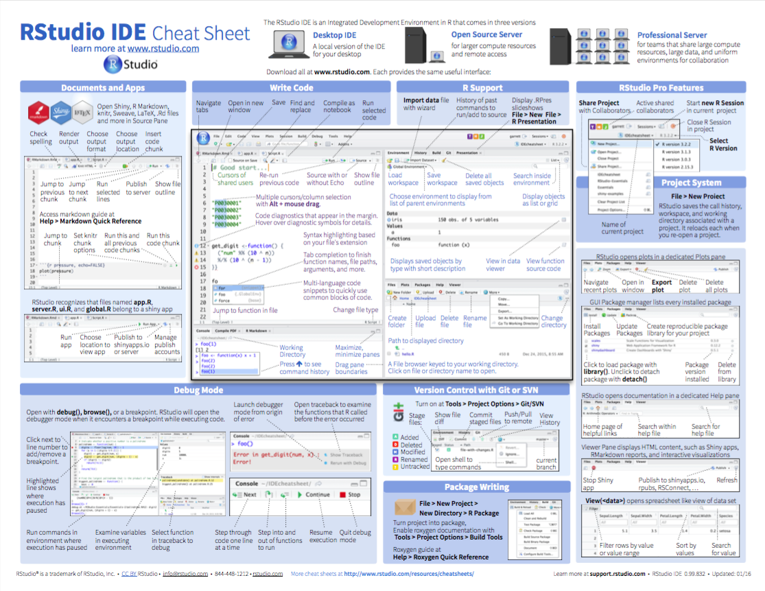
Figure 2.6: RStudio IDE cheat sheet.
2.4.6 Knowledge check
- Identify which working directory you are working out of.
- Create a folder on your computer titled Learning R. Within RStudio, set your working directory to this folder.
-
Type
piin the console. Set the option to show 8 digits. Re-typepiin the console. -
Type
?piin the console. Note that documentation on this object pops up in the Help tab in the Misc. Display. - Now check out your code History tab.
-
Create a new .R file and save this as my-first-script (note
how this now appears in your Learning R folder). Type
piin line 1 of this script,options(digits = 8)in line 2, andpiagain in line three. Execute this code one line at a time and then re-execute all lines at once.
2.5 Getting help
The help documentation and support in R is comprehensive and easily accessible from the the console.
2.5.1 General Help
To leverage general help resources you can use:
# provides general help links
help.start()

# searches the help system for documentation matching a given character string
help.search("linear regression")
Note that the help.search("some text here") function requires a character string enclosed in quotation marks. So if you are in search of time series functions in R, using help.search("time series") will pull up a healthy list of vignettes and code demonstrations that illustrate packages and functions that work with time series data.
For more direct help on functions that are installed on your computer you can use the following. Test these out in your console:
help(mean)      # provides details for specific function
?mean           # provides same information as help(functionname)
example(mean)   # provides examples for said function
Note that the help() and ? function calls only work for functions within loaded packages. You’ll understand what this means shortly.
2.5.2 Getting Help From the Web
Typically, a problem you may be encountering is not new and others have faced, solved, and documented the same issue online. The following resources can be used to search for online help. Although, I typically just Google the problem and find answers relatively quickly.
RSiteSearch("key phrase"): searches for the key phrase in help manuals and archived mailing lists on the R Project website.- Stack Overflow: a searchable Q&A site oriented toward programming issues. 75% of my answers typically come from Stack Overflow.
- Cross Validated: a searchable Q&A site oriented toward statistical analysis.
- RStudio Community: a community for all things R and RStudio where you can get direct answers to your problems and also give back by helping to solve and answer other’s questions.
- R-seek: a Google custom search that is focused on R-specific websites
- R-bloggers: a central hub of content collected from over 500 bloggers who provide news and tutorials about R.
Twitter has a thriving R community (#rstats) and is definitely worth following. However, it is not the place to ask for help on specific code functionality.
2.5.3 Knowledge check
-
Does
help.start()provide a link to an introduction to R manual? -
Does R’s
modefunction compute the statistical mode? - Review at least 5 Stack Overflow questions about R.
2.6 Errors, warnings, and messages
One thing that intimidates new R users (and new programmers in general) is when they run into errors, warnings, and messages. R reports errors, warnings, and messages in the following way. Don’t worry about what the code is doing, just get familiar with the differences in how errors, warnings, and messages are reported.
Errors: When the red text is a legitimate error, it will be prefaced with “Error in…” and will try to explain what went wrong. Generally when there’s an error, the code will not run. Think of errors as a red traffic light: something is wrong!
For references on common errors, check out the following links by Noam Ross, David Smith, and Chester Ismay.
Warnings: Warning messages will be prefaced with “Warning:” and R will try to explain why there’s a warning. Generally your code will still work, but with some caveats. Think of warnings as a yellow traffic light: everything is working, but watch out/pay attention. Typically when you get a warning you want to figure out what is throwing the warning because the end result may not be what you had intended!
Messages: When the text doesn’t start with either “Error” or “Warning”, it’s just a friendly message. You’ll often see these messages when you load R packages or make certain function calls. Think of messages as a green traffic light: everything is working fine and keep on going!
References
You can access this tutorial at http://dss.princeton.edu/training/RStudio101.pdf. Note that although it is from 2013 it still is very applicable and does a very thorough introduction↩︎
You can assess the script editor tutorial at https://support.rstudio.com/hc/en-us/articles/200484448-Editing-and-Executing-Code↩︎