12 Lesson 3c: Tidy data
“Cannot emphasize enough how much time you save by putting analysis efforts into tidying data first.” - Hilary Parker
Jenny Bryan stated that “classroom data are like teddy bears and real data are like a grizzley bear with salmon blood dripping out its mouth.” In essence, she was getting to the point that often when we learn how to perform a modeling approach in the classroom, the data used is provided in a format that appropriately feeds into the modeling tool of choice. In reality, datasets are messy and “every messy dataset is messy in its own way.”7 The concept of “tidy data” was established by Hadley Wickham and represents a “standardized way to link the structure of a dataset (its physical layout) with its semantics (its meaning).”8 The objective should always to be to get a dataset into a tidy form which consists of:
- Each variable forms a column
- Each observation forms a row
- Each type of observational unit forms a table
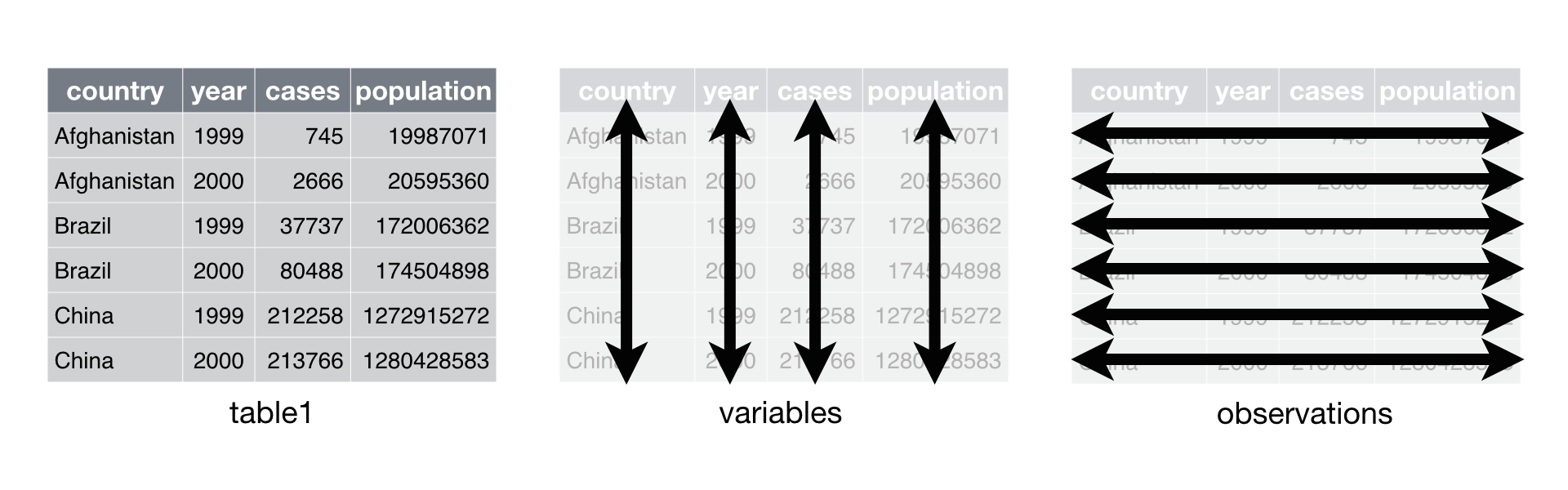
Figure 12.1: Tidy data.
To create tidy data you need to be able to reshape your data; preferably via efficient and simple code. To help with this process Hadley created the tidyr package. This lesson covers the basics of tidyr to help you reshape your data as necessary.
If you’d like to learn more about the underlying theory, you might enjoy the Tidy Data paper published in the Journal of Statistical Software, http://www.jstatsoft.org/v59/i10/paper.
12.1 Learning objectives
Upon completing this module you will be able to:
- Make wide data long and long data wide.
- Separate and combine parts of columns.
- Impute missing values
Note: Some of the data used in the recorded lectures are different then those used in this chapter. If you want to follow along with the recordings be sure to download the supplementary data files, which can be found in canvas.
12.2 Prerequisites
Load the tidyr package to provide you access to the functions we’ll cover in this lesson. We’ll also use dplyr for a few examples.
To illustrate various tidying tasks we will use several untidy datasets provided in the data directory (or via Canvas material download).
These are artificial customer transaction datasets that are designed to mimick actual data.
12.3 Making wide data longer
There are times when our data is considered “wide” or “unstacked” and a common attribute/variable of concern is spread out across columns. To reformat the data such that these common attributes are gathered together as a single variable, the pivot_longer() function will take multiple columns and collapse them into key-value pairs, duplicating all other columns as needed.
For example, let’s say we have the given data frame.
(untidy1 <- readr::read_csv("data/untidy1.csv"))
## Rows: 3144 Columns: 5
## ── Column specification ───────────────────────────────────────────────
## Delimiter: ","
## chr (1): prod_desc
## dbl (4): hshd_id, Mar, Apr, May
##
## ℹ Use `spec()` to retrieve the full column specification for this data.
## ℹ Specify the column types or set `show_col_types = FALSE` to quiet this message.
## # A tibble: 3,144 × 5
##       hshd_id prod_desc                   Mar   Apr   May
##         <dbl> <chr>                     <dbl> <dbl> <dbl>
##  1 3376002291 HNTS MEAT FLV PASTA SAUCE  1     0     0
##  2 3376163223 RAGU SPICY ITL STYL SAUCE  1.89  0     0
##  3 3376542041 HMK CARD MDAY MOTHER       0     0     5.29
##  4 3377032853 HMK CARD BRTHDAY CROWN     3.99  0     0
##  5 3377032853 MZTA MARINARA PASTA SAUCE  8.78  0     0
##  6 3377285583 HMK CARD ADMIN ANYONE      0     2     0
##  7 3377285583 HMK CARD MDAY              0     0     4.99
##  8 3377285583 HMK CARD MDAY ANYONE       0     3.99  0
##  9 3377285583 HMK CARD MDAY MOTHER       0     2.99  7.99
## 10 3377285583 SLV PLT TOMTO MARNARA SCE  8.97  0     0
## # ℹ 3,134 more rows
This data is considered untidy in the wide sense since the month variable is structured such that each month represents a variable. If we wanted to compute the total amount each household spent by month, this data set does not provide a convenient shape to work with. To re-structure the month component as an individual variable, we can pivot this data to be longer such that each month is within one column variable and the values associated with each month in a second column variable.
untidy1 %>%
   pivot_longer(cols = Mar:May, names_to = "month", values_to = "net_spend_amt")
## # A tibble: 9,432 × 4
##       hshd_id prod_desc                 month net_spend_amt
##         <dbl> <chr>                     <chr>         <dbl>
##  1 3376002291 HNTS MEAT FLV PASTA SAUCE Mar            1
##  2 3376002291 HNTS MEAT FLV PASTA SAUCE Apr            0
##  3 3376002291 HNTS MEAT FLV PASTA SAUCE May            0
##  4 3376163223 RAGU SPICY ITL STYL SAUCE Mar            1.89
##  5 3376163223 RAGU SPICY ITL STYL SAUCE Apr            0
##  6 3376163223 RAGU SPICY ITL STYL SAUCE May            0
##  7 3376542041 HMK CARD MDAY MOTHER      Mar            0
##  8 3376542041 HMK CARD MDAY MOTHER      Apr            0
##  9 3376542041 HMK CARD MDAY MOTHER      May            5.29
## 10 3377032853 HMK CARD BRTHDAY CROWN    Mar            3.99
## # ℹ 9,422 more rows
This new structure allows us to perform follow-on analysis in a much easier fashion. For example, if we wanted to compute the total amount each household spent by month, we could simply do the following sequence:
untidy1 %>%
   pivot_longer(cols = Mar:May, names_to = "month", values_to = "net_spend_amt") %>%
   group_by(hshd_id, month) %>%
   summarize(monthly_spend = sum(net_spend_amt))
## # A tibble: 3,708 × 3
## # Groups:   hshd_id [1,236]
##       hshd_id month monthly_spend
##         <dbl> <chr>         <dbl>
##  1 3376002291 Apr            0
##  2 3376002291 Mar            1
##  3 3376002291 May            0
##  4 3376163223 Apr            0
##  5 3376163223 Mar            1.89
##  6 3376163223 May            0
##  7 3376542041 Apr            0
##  8 3376542041 Mar            0
##  9 3376542041 May            5.29
## 10 3377032853 Apr            0
## # ℹ 3,698 more rows
It’s important to note that there is flexibility in how you specify the columns you would like to gather. In our example we used cols = Mar:May to imply we want to use all the columns including and between Mar and May. We could also have used the following to produce the same results:
untidy1 %>% pivot_longer(cols = Mar:May, names_to = "month", values_to = "net_spend_amt")
untidy1 %>% pivot_longer(cols = c(Mar, Apr, May), names_to = "month", values_to = "net_spend_amt")
untidy1 %>% pivot_longer(cols = 3:5, names_to = "month", values_to = "net_spend_amt")
untidy1 %>% pivot_longer(cols = -c(hshd_id, prod_desc), names_to = "month", values_to = "net_spend_amt")
12.3.1 Knowledge check
Using the data provided by tidyr::table4b:
- Is this data untidy? If so, why?
- Compute the sum of the values across the years for each country.
- Now pivot this data set so that it is tidy with the year values represented in their own column called ‘year’ and the values listed in their own ‘population’ column.
- Using the pipe operator to chain together a sequence of functions, perform #3 and then compute the mean population for each country.
12.4 Making long data wider
There are also times when we are required to turn long formatted data into wide formatted data – in other words, we want to pivot data to be wider. As a complement to pivot_longer, the pivot_wider function spreads a key-value pair across multiple columns. For example, the given data frame captures total household purchases for each product along with the household’s shopping habit (Premium Loyal, Valuable, etc.).
(untidy2 <- readr::read_csv("data/untidy2.csv"))
## Rows: 1536 Columns: 4
## ── Column specification ───────────────────────────────────────────────
## Delimiter: ","
## chr (2): shabit, prod_merch_l20_desc
## dbl (2): hshd_id, net_spend_amt
##
## ℹ Use `spec()` to retrieve the full column specification for this data.
## ℹ Specify the column types or set `show_col_types = FALSE` to quiet this message.
## # A tibble: 1,536 × 4
##       hshd_id shabit        prod_merch_l20_desc net_spend_amt
##         <dbl> <chr>         <chr>                       <dbl>
##  1 3376002291 Valuable      PASTA & PIZZA SAUCE          1
##  2 3376163223 Premium Loyal PASTA & PIZZA SAUCE          1.89
##  3 3376542041 Potential     GREETING CARDS               5.29
##  4 3377032853 Uncommitted   GREETING CARDS               3.99
##  5 3377032853 Uncommitted   PASTA & PIZZA SAUCE          8.78
##  6 3377285583 Premium Loyal GREETING CARDS              22.0
##  7 3377285583 Premium Loyal PASTA & PIZZA SAUCE         11.4
##  8 3377528247 Valuable      GREETING CARDS              11.0
##  9 3378020265 Valuable      GREETING CARDS               6.99
## 10 3379767653 Uncommitted   GREETING CARDS               3.99
## # ℹ 1,526 more rows
Currently, this data set is in a tidy format. But say we wanted to perform a classification model where we try to use the amount spent on each product to predict the shopping habit of each household, we would need to reorganize the data to make it compatible with future algorithms. To address this, we would need to pivot this data such that each product as its own variable with the total dollar amount spent on each product as the values. In essence, we are transposing the values in prod_merch_l20_desc to be the new variable names (aka key) and then adding the values in net_spend_amt to be the value under each variable name.
untidy2 %>%
   pivot_wider(names_from = prod_merch_l20_desc, values_from = net_spend_amt)
## # A tibble: 1,236 × 5
##       hshd_id shabit        `PASTA & PIZZA SAUCE` `GREETING CARDS`
##         <dbl> <chr>                         <dbl>            <dbl>
##  1 3376002291 Valuable                       1               NA
##  2 3376163223 Premium Loyal                  1.89            NA
##  3 3376542041 Potential                     NA                5.29
##  4 3377032853 Uncommitted                    8.78             3.99
##  5 3377285583 Premium Loyal                 11.4             22.0
##  6 3377528247 Valuable                      NA               11.0
##  7 3378020265 Valuable                      NA                6.99
##  8 3379767653 Uncommitted                    2.19             3.99
##  9 3379815863 Premium Loyal                  1.49            NA
## 10 3380253171 Uncommitted                   NA                7.99
## # ℹ 1,226 more rows
## # ℹ 1 more variable: `NF SHORTENING AND OIL` <dbl>
This results in each household (hshd_id) having its own observation. You probably notice that there are now a lot of missing values which causes NA to be populated. If you were to apply this data to one of the many machine learning algorithms, you would likely run into errors due to the NAs. In this example, we could replace those NAs with zeros using values_fill = 0, since the household did not purchase any of those products.
untidy2 %>%
   pivot_wider(names_from = prod_merch_l20_desc, values_from = net_spend_amt, values_fill = 0)
## # A tibble: 1,236 × 5
##       hshd_id shabit        `PASTA & PIZZA SAUCE` `GREETING CARDS`
##         <dbl> <chr>                         <dbl>            <dbl>
##  1 3376002291 Valuable                       1                0
##  2 3376163223 Premium Loyal                  1.89             0
##  3 3376542041 Potential                      0                5.29
##  4 3377032853 Uncommitted                    8.78             3.99
##  5 3377285583 Premium Loyal                 11.4             22.0
##  6 3377528247 Valuable                       0               11.0
##  7 3378020265 Valuable                       0                6.99
##  8 3379767653 Uncommitted                    2.19             3.99
##  9 3379815863 Premium Loyal                  1.49             0
## 10 3380253171 Uncommitted                    0                7.99
## # ℹ 1,226 more rows
## # ℹ 1 more variable: `NF SHORTENING AND OIL` <dbl>
12.4.1 Knowledge check
Using the data provided by tidyr::table2:
- Is this data untidy? If so, why?
- Compute the cases-to-population ratio for each country by year.
-
Now pivot this data set so that it is tidy with 4 columns:
country,year,cases, andpopulation. - Using the pipe operator to chain together a sequence of functions, perform #3 and then compute the cases-to-population ratio for each country by year.
12.5 Separate one variable into multiple
Many times a single column variable will capture multiple variables, or even parts of a variable you just don’t care about. This is exemplified in the following untidy3 data frame. Here, the product variable combines two variables, the product category (i.e. greeting cards, Pasta & pizza sauce) along with the product description (i.e. graduation cards, birthday cards). For many reasons (summary statistics, visualization, modeling) we would likely want to separate these parts into their own variables.
(untidy3 <- readr::read_csv("data/untidy3.csv"))
## Rows: 3884 Columns: 4
## ── Column specification ───────────────────────────────────────────────
## Delimiter: ","
## chr (2): shabit, product
## dbl (2): hshd_id, net_spend_amt
##
## ℹ Use `spec()` to retrieve the full column specification for this data.
## ℹ Specify the column types or set `show_col_types = FALSE` to quiet this message.
## # A tibble: 3,884 × 4
##       hshd_id shabit        net_spend_amt product
##         <dbl> <chr>                 <dbl> <chr>
##  1 8614328969 Premium Loyal          0.99 GREETING CARDS: CREPE
##  2 8614328969 Premium Loyal          0.99 GREETING CARDS: CREPE
##  3 3479082131 Premium Loyal          1.89 GREETING CARDS: CREPE
##  4 3479082131 Premium Loyal          1.89 GREETING CARDS: CREPE
##  5 3479082131 Premium Loyal          1.89 GREETING CARDS: CREPE
##  6 3479082131 Premium Loyal          1.89 GREETING CARDS: CREPE
##  7 5003651017 Uncommitted            1.89 GREETING CARDS: CREPE
##  8 5003651017 Uncommitted            1.89 GREETING CARDS: CREPE
##  9 5003651017 Uncommitted            1.89 GREETING CARDS: CREPE
## 10 8614328969 Premium Loyal          1.49 GREETING CARDS: BALLOONS
## # ℹ 3,874 more rows
This can be accomplished using the separate function which separates a single column into multiple columns based on a separator. Additional arguments provide some flexibility with separating columns.
# separate product column into two variables named "prod_category" & "prod_desc"
untidy3 %>%
   separate(col = product, into = c("prod_category", "prod_desc"), sep = ": ")
## # A tibble: 3,884 × 5
##       hshd_id shabit        net_spend_amt prod_category  prod_desc
##         <dbl> <chr>                 <dbl> <chr>          <chr>
##  1 8614328969 Premium Loyal          0.99 GREETING CARDS CREPE
##  2 8614328969 Premium Loyal          0.99 GREETING CARDS CREPE
##  3 3479082131 Premium Loyal          1.89 GREETING CARDS CREPE
##  4 3479082131 Premium Loyal          1.89 GREETING CARDS CREPE
##  5 3479082131 Premium Loyal          1.89 GREETING CARDS CREPE
##  6 3479082131 Premium Loyal          1.89 GREETING CARDS CREPE
##  7 5003651017 Uncommitted            1.89 GREETING CARDS CREPE
##  8 5003651017 Uncommitted            1.89 GREETING CARDS CREPE
##  9 5003651017 Uncommitted            1.89 GREETING CARDS CREPE
## 10 8614328969 Premium Loyal          1.49 GREETING CARDS BALLOONS
## # ℹ 3,874 more rows
The default separator is any non alpha-numeric character. In this
example there are two: white space ” “ and colon
: so we need to specify. You can also keep the original
column that you are separating by including
remove = FALSE.
You can also pass a vector of integers to sep and separate() will interpret the integers as positions to split at. For example, say our household ID (hshd_id) value actually represents the the household and user. So, let’s say the first 7 digits is the household identifier and the last 3 digits is the user identifier. We can split this into two new variables with the following:
untidy3 %>%
   separate(hshd_id, into = c("hshd_id", "member_id"), sep = 7)
## # A tibble: 3,884 × 5
##    hshd_id member_id shabit        net_spend_amt product
##    <chr>   <chr>     <chr>                 <dbl> <chr>
##  1 8614328 969       Premium Loyal          0.99 GREETING CARDS: CREPE
##  2 8614328 969       Premium Loyal          0.99 GREETING CARDS: CREPE
##  3 3479082 131       Premium Loyal          1.89 GREETING CARDS: CREPE
##  4 3479082 131       Premium Loyal          1.89 GREETING CARDS: CREPE
##  5 3479082 131       Premium Loyal          1.89 GREETING CARDS: CREPE
##  6 3479082 131       Premium Loyal          1.89 GREETING CARDS: CREPE
##  7 5003651 017       Uncommitted            1.89 GREETING CARDS: CREPE
##  8 5003651 017       Uncommitted            1.89 GREETING CARDS: CREPE
##  9 5003651 017       Uncommitted            1.89 GREETING CARDS: CREPE
## 10 8614328 969       Premium Loyal          1.49 GREETING CARDS: BALLO…
## # ℹ 3,874 more rows
You can use positive and negative values to split the column. Positive values start at 1 on the far-left of the strings; negative value start at -1 on the far-right of the strings.
12.5.1 Knowledge check
Using the data provided by tidyr::table3:
- Is this data untidy? If so, why?
-
The
ratevariable is actually combining the number of cases and the population. Split this column such that you have four columns:country,year,cases, andpopulation. - Using the pipe operator to chain together a sequence of functions, perform #2 and then compute the cases-to-population ratio for each country by year.
12.6 Combine multiple variables into one
Similarly, there are times when we would like to combine the values of two variables. As a compliment to separate, the unite function is a convenient function to paste together multiple variable values into one. Consider the following data frame that has separate date variables. To perform time series analysis or for visualizations we may desire to have a single date column.
(untidy4 <- readr::read_csv("data/untidy4.csv"))
## Rows: 3884 Columns: 7
## ── Column specification ───────────────────────────────────────────────
## Delimiter: ","
## chr (2): shabit, prod_desc
## dbl (5): hshd_id, net_spend_amt, year, month, day
##
## ℹ Use `spec()` to retrieve the full column specification for this data.
## ℹ Specify the column types or set `show_col_types = FALSE` to quiet this message.
## # A tibble: 3,884 × 7
##       hshd_id shabit        net_spend_amt prod_desc  year month   day
##         <dbl> <chr>                 <dbl> <chr>     <dbl> <dbl> <dbl>
##  1 8614328969 Premium Loyal          0.99 CREPE      2017     5    30
##  2 8614328969 Premium Loyal          0.99 CREPE      2017     5    30
##  3 3479082131 Premium Loyal          1.89 CREPE      2017     3     6
##  4 3479082131 Premium Loyal          1.89 CREPE      2017     3     6
##  5 3479082131 Premium Loyal          1.89 CREPE      2017     3     6
##  6 3479082131 Premium Loyal          1.89 CREPE      2017     3     6
##  7 5003651017 Uncommitted            1.89 CREPE      2017     3    28
##  8 5003651017 Uncommitted            1.89 CREPE      2017     3    28
##  9 5003651017 Uncommitted            1.89 CREPE      2017     3    28
## 10 8614328969 Premium Loyal          1.49 BALLOONS   2017     5    30
## # ℹ 3,874 more rows
We can accomplish this by uniting these columns into one variable with unite.
untidy4 %>% unite(col = "date", year:day, sep = "-")
## # A tibble: 3,884 × 5
##       hshd_id shabit        net_spend_amt prod_desc date
##         <dbl> <chr>                 <dbl> <chr>     <chr>
##  1 8614328969 Premium Loyal          0.99 CREPE     2017-5-30
##  2 8614328969 Premium Loyal          0.99 CREPE     2017-5-30
##  3 3479082131 Premium Loyal          1.89 CREPE     2017-3-6
##  4 3479082131 Premium Loyal          1.89 CREPE     2017-3-6
##  5 3479082131 Premium Loyal          1.89 CREPE     2017-3-6
##  6 3479082131 Premium Loyal          1.89 CREPE     2017-3-6
##  7 5003651017 Uncommitted            1.89 CREPE     2017-3-28
##  8 5003651017 Uncommitted            1.89 CREPE     2017-3-28
##  9 5003651017 Uncommitted            1.89 CREPE     2017-3-28
## 10 8614328969 Premium Loyal          1.49 BALLOONS  2017-5-30
## # ℹ 3,874 more rows
Don’t worry, we’ll learn more appropriate ways to deal with dates in a later lesson.
12.6.1 Knowledge check
Using the data provided by tidyr::table5:
- Is this data untidy? If so, why?
-
Unite and separate the necessary columns such that you have four
columns:
country,year,cases, andpopulation. - Using the pipe operator to chain together a sequence of functions, perform #2 and then compute the cases-to-population ratio for each country by year.
12.7 Additional tidying functions
The previous four functions (pivot_longer, pivot_wider, separate and unite) are the primary functions you will find yourself using on a continuous basis; however, there are some handy functions that are lesser known with the tidyr package. Consider this untidy data frame.
expenses <- tibble::as_tibble(read.table(header = TRUE, text = "
        Dept    Year   Month   Day         Cost
           A    2015      01    01      $500.00
          NA      NA      02    05       $90.00
          NA      NA      02    22    $1,250.45
          NA      NA      03    NA      $325.10
           B      NA      01    02      $260.00
          NA      NA      02    05       $90.00
", stringsAsFactors = FALSE))
Often Excel reports will not repeat certain variables. When we read these reports in, the empty cells are typically filled in with NA such as in the Dept and Year columns of our expense data frame. We can fill these values in with the previous entry using fill():
expenses %>% fill(Dept, Year)
## # A tibble: 6 × 5
##   Dept   Year Month   Day Cost
##   <chr> <int> <int> <int> <chr>
## 1 A      2015     1     1 $500.00
## 2 A      2015     2     5 $90.00
## 3 A      2015     2    22 $1,250.45
## 4 A      2015     3    NA $325.10
## 5 B      2015     1     2 $260.00
## 6 B      2015     2     5 $90.00
Also, sometimes accounting values in Excel spreadsheets get read in as a character value, which is the case for the Cost variable. We may wish to extract only the numeric part of this regular expression, which can be done with readr::parse_number. Note that parse_number works on a single variable so when you pipe the expense data frame into the function you need to use %$% operator as discussed in the Pipe Operator lesson.
library(magrittr)

expenses %$% readr::parse_number(Cost)
## [1]  500.0   90.0 1250.5  325.1  260.0   90.0

# you can use this to convert and save the Cost column to a numeric variable
expenses %>% dplyr::mutate(Cost = readr::parse_number(Cost))
## # A tibble: 6 × 5
##   Dept   Year Month   Day  Cost
##   <chr> <int> <int> <int> <dbl>
## 1 A      2015     1     1  500
## 2 <NA>     NA     2     5   90
## 3 <NA>     NA     2    22 1250.
## 4 <NA>     NA     3    NA  325.
## 5 B        NA     1     2  260
## 6 <NA>     NA     2     5   90
You can also easily replace missing (or NA) values with a specified value:
# replace the missing Day value
expenses %>% replace_na(replace = list(Day = 31))
## # A tibble: 6 × 5
##   Dept   Year Month   Day Cost
##   <chr> <int> <int> <int> <chr>
## 1 A      2015     1     1 $500.00
## 2 <NA>     NA     2     5 $90.00
## 3 <NA>     NA     2    22 $1,250.45
## 4 <NA>     NA     3    31 $325.10
## 5 B        NA     1     2 $260.00
## 6 <NA>     NA     2     5 $90.00

# replace both the missing Day and Year values
expenses %>% replace_na(replace = list(Year = 2015, Day = 31))
## # A tibble: 6 × 5
##   Dept   Year Month   Day Cost
##   <chr> <int> <int> <int> <chr>
## 1 A      2015     1     1 $500.00
## 2 <NA>   2015     2     5 $90.00
## 3 <NA>   2015     2    22 $1,250.45
## 4 <NA>   2015     3    31 $325.10
## 5 B      2015     1     2 $260.00
## 6 <NA>   2015     2     5 $90.00
12.8 Putting it altogether
Since the %>% operator is embedded in tidyr, we can string multiple operations together to efficiently tidy data and make the process easy to read and follow. To illustrate, let’s use the following data, which has multiple messy attributes.
a_mess <- tibble::as_tibble(read.table(header = TRUE, text = "
   Dep_Unt   Year     Q1     Q2     Q3     Q4
    A.1      2006     15     NA     19     17
    B.1        NA     12     13     27     23
    A.2        NA     22     22     24     20
    B.2        NA     12     13     25     18
    A.1      2007     16     14     21     19
    B.2        NA     13     11     16     15
    A.2        NA     23     20     26     20
    B.2        NA     11     12     22     16
"))
In this case, a tidy data set should result in columns of Dept, Unit, Year, Quarter, and Cost. Furthermore, we want to fill in the year column where NAs currently exist. And we’ll assume that we know the missing value that exists in the Q2 column, and we’d like to update it.
a_mess %>%
  fill(Year) %>%
  pivot_longer(cols = Q1:Q4, names_to = "Quarter", values_to = "Cost") %>%
  separate(Dep_Unt, into = c("Dept", "Unit")) %>%
  replace_na(replace = list(Cost = 17))
## # A tibble: 32 × 5
##    Dept  Unit   Year Quarter  Cost
##    <chr> <chr> <int> <chr>   <int>
##  1 A     1      2006 Q1         15
##  2 A     1      2006 Q2         17
##  3 A     1      2006 Q3         19
##  4 A     1      2006 Q4         17
##  5 B     1      2006 Q1         12
##  6 B     1      2006 Q2         13
##  7 B     1      2006 Q3         27
##  8 B     1      2006 Q4         23
##  9 A     2      2006 Q1         22
## 10 A     2      2006 Q2         22
## # ℹ 22 more rows
12.9 Exercises
- Is the following data set “tidy”? Why or why not?
people <- tribble(
  ~name,             ~names,  ~values,
  #-----------------|--------|------
  "Phillip Woods",   "age",       45,
  "Phillip Woods",   "height",   186,
  "Phillip Woods",   "age",       50,
  "Jessica Cordero", "age",       37,
  "Jessica Cordero", "height",   156
)- Using the data set above, convert the “name” column into “first_name” and “last_name” columns.
- Now pivot this data set such that the “names” and “values” columns are converted into “age” and “height” columns.