22 Lesson 6a: Conditional statements
Conditional statements are a key part of any programming language. Their purpose is to evaluate if some condition holds and then execute a particular task depending on the result. In this lesson we’ll perform some basic if and if-else conditional assessments and then build on those by adding multiple conditional assessments and also look at vectorized approaches.
22.1 Learning objectives
By the end of this lesson you will be able to:
- Apply basic
ifandif...elsestatements. - Add multiple conditional assessments.
- Apply non-vectorized and vectorized conditional statements.
- Incorporate these approaches for data mining data frames.
22.2 Prerequisites
Many base R functions exist to perform control statements; however, we can also perform extensions of control statements using functions in the tidyverse package.
To illustrate various control tasks we will use the Complete Journey customer transaction data.
22.3 if statement
The conditional if statement is used to test an expression. If the test_expression is TRUE, the statement gets executed. But if it’s FALSE, nothing happens.
Say, for example, that we want R to print a message depending on the value of x:
If the condition is TRUE then the statement within the brackets is executed:
if (x > .5) {
  paste("x equals", round(x, 2), "which is greater than 0.5")
}
## [1] "x equals 0.51 which is greater than 0.5"
However, if the condition is FALSE then the statement is not executed:
Now say you have a vector of values that you would like to test. One would think you would just perform the following; however, you can see that you will get an error:
x <- c(8, 3, -2, 5)

if (x < 0) {
  print("x contains a negative number")
}
## Error in if (x < 0) {: the condition has length > 1
This is because if() is not vectorized and it seeks to assess a single logical condition.
To assess if a condition holds among multiple inputs, use any() or all().
any() looks to see if at least one value in the vector meets the condition:
any(x < 0)
## [1] TRUE

if(any(x < 0)) {
  print("x contains a negative number")
}
## [1] "x contains a negative number"
While all() looks to see if all values in the vector meets the condition:
There are actually two ways to write this if statement;
since the body of the statement is only one line you can write it with
or without curly braces. I recommend getting in the habit of using curly
braces, that way if you build onto if statements with
additional functions in the body or add an else statement
later you will not run into issues with unexpected code procedures.
# without curly braces
if(any(x < 0)) print("x contains negative numbers")
## [1] "x contains negative numbers"

# with curly braces produces same result
if (any(x < 0)) {
   print("x contains negative numbers")
}
## [1] "x contains negative numbers"
22.4 ifelse statement
The conditional if...else statement is used to test an expression similar to the if statement. However, rather than nothing happening if the test_expression is FALSE, the else part of the function will be evaluated.
The following extends the if example illustrated in the previous section. Here, the if...else statement tests if any values in a vector are negative; if TRUE it produces one output and if FALSE it produces the else output.
# this test results in statement 1 being executed
x <- c(8, 3, -2, 5)
if (any(x < 0)) {
print("x contains negative numbers")
} else {
print("x contains all positive numbers")
}
## [1] "x contains negative numbers"
# this test results in statement 2 (or the else statement) being executed
y <- c(8, 3, 2, 5)
if (any(y < 0)) {
print("y contains negative numbers")
} else {
print("y contains all positive numbers")
}
## [1] "y contains all positive numbers"
22.4.1 Knowledge check
Fill in the following code chunk so that:
- if month has value 1-9 the file name printed out will be “data/month-0X.csv”
- if month has value 10-12 the file name printed out will be “data/month-1X.csv”
- test it out for when month equals 4, 6, 10, & 12
month <- 4

if (month _____) {
  paste0("data/", "Month-0", month, ".csv")
} else {
paste0("data/", "Month-", month, ".csv")
}
22.5 Multiple conditions
We can continue to expand an if...else statement to assess more than just binary conditions by incorporating else if steps:
x <- 0

if (x < 0) {
   print("x is a negative number")
} else if (x > 0) {
   print("x is a positive number")
} else {
   print("x is zero")
}
## [1] "x is zero"
Note how we extend by following else with
if(). But we should always end with an
else.
22.5.1 Knowledge check
Fill in the following code chunk so that:
- if month has value 1-9 the file name printed out will be “data/month-0X.csv”
- if month has value 10-12 the file name printed out will be “data/month-1X.csv”
- if month is an invalid month number (not 1-12), the result printed out is “Invalid month”
- test it out for when month equals 6, 10, & 13
month <- 4

if (month _____) {
   paste0("data/", "Month-0", month, ".csv")
} else if (month _____) {
   paste0("data/", "Month-", month, ".csv")
} else {
   print("_____")
}
22.6 Vectorized approaches
So far, we have focused on controlling the flow based on a single conditional statement. Basically, given one element we assess if that element meets a certain condition or multiple elements we simply assess if the condition holds for all/any elements:
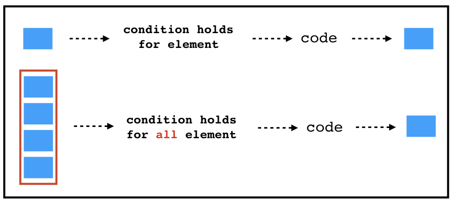
Figure 22.1: Illustration of non-vectorized conditional statements.
However, what if we want to assess the condition against each element and execute code if that condition is TRUE for each element (aka vectorized)?
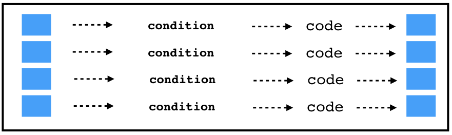
Figure 22.2: Illustration of vectorized conditional statements.
We can vectorize an if...else statement a couple of ways. One option is to use the ifelse() function built in base R:
(x <- c(runif(5), NA))
## [1] 0.306769 0.426908 0.693102 0.085136 0.225437       NA

ifelse(x > .5, "greater than", "less than")
## [1] "less than"    "less than"    "greater than" "less than"
## [5] "less than"    NA
Second, we can use dplyr::if_else(), which provides a little more stability in output type and flexibility in what to do with missing values:
if_else(x > .5, "greater than", "less than", missing = "something else")
## [1] "less than"      "less than"      "greater than"   "less than"
## [5] "less than"      "something else"
However, in both cases, they can only assess binary conditional statements. If we want to vectorize multiple conditions (i.e. if...else...if...else) then the best approach is to use dplyr::case_when().
The syntax for case_when() can be a little confusing at first. Basically, a conditional expression looks like condition ~ code to execute. Consequently:
x < .3is the first condition to assess and if it isTRUEthen the result is what comes after the~.- If the first condition is not met, then
case_whenwill evaluate the second, third, etc. until it finds a condition that is true. - If you include
TRUE ~ some_expressionat the end then any element that does not meet a prior condition will be consideredTRUEand the expression will be evaluated. So in the below code, any element that doesn’t meet the prior conditions will be lumped into an “out of bounds” category.
set.seed(123)
(x <- c(runif(10), NA, Inf, 1.25))
##  [1] 0.287578 0.788305 0.408977 0.883017 0.940467 0.045556 0.528105
##  [8] 0.892419 0.551435 0.456615       NA      Inf 1.250000

dplyr::case_when(
  x < .3   ~ "low",
  x < .7   ~ "medium",
  x < .9   ~ "medium high",
  x <=1.0  ~ "high",
  is.na(x) ~ "missing",
  TRUE     ~ "out of bounds"
)
##  [1] "low"           "medium high"   "medium"        "medium high"
##  [5] "high"          "low"           "medium"        "medium high"
##  [9] "medium"        "medium"        "missing"       "out of bounds"
## [13] "out of bounds"
22.7 With data frames
So how can we leverage these skills when performing exploratory data analysis? Most common is to use use ifelse(), if_else(), and case_when() within dplyr::mutate().
For example, say we want to create a new variable that classifies transactions above $10 as “high value” otherwise they are “low value”. We can use the dplyr::if_else function within mutate to perform this.
# I use select simply to reduce the size of the data set so you can easily
# see results
transactions %>%
   select(household_id, basket_id, sales_value) %>%
   mutate(value = if_else(sales_value > 10, 'high value', 'low value'))
## # A tibble: 75,000 × 4
##    household_id basket_id   sales_value value
##    <chr>        <chr>             <dbl> <chr>
##  1 2261         31625220889        3.86 low value
##  2 2131         32053127496        1.59 low value
##  3 511          32445856036        1    low value
##  4 400          31932241118       11.9  high value
##  5 918          32074655895        1.29 low value
##  6 718          32614612029        2.5  low value
##  7 868          32074722463        3.49 low value
##  8 1688         34850403304        2    low value
##  9 467          31280745102        6.55 low value
## 10 1947         32744181707        3.99 low value
## # ℹ 74,990 more rows
dplyr::if_else is preferred to the base R
ifelse function because it allows you to work with missing
values more conveniently.
When we want to perform multiple if_else statements within mutate we can embed multiple if_else statements within each other. Unfortunately, this gets pretty confusing quickly so a more convenient approach is to use case_when. For example, we can create a new variable that results in the following:
- Large purchase:
quantity > 20orsales_value > 10
- Medium purchase:
quantity > 10orsales_value > 5 - small purchase:
quantity > 0orsales_value > 0 - Alternative transaction: all other transactions
# I use select simply to reduce the size of the data set so you can easily
# see results
transactions %>%
   select(household_id, basket_id, quantity, sales_value) %>%
   mutate(
     value = case_when(
       quantity > 20 | sales_value > 10 ~ "Large purchase",
       quantity > 10 | sales_value > 5  ~ "Medium purchase",
       quantity > 0 | sales_value > 0  ~ "Small purchase",
       TRUE ~ "Alternative transaction"
     )
   )
## # A tibble: 75,000 × 5
##    household_id basket_id   quantity sales_value value
##    <chr>        <chr>          <dbl>       <dbl> <chr>
##  1 2261         31625220889        1        3.86 Small purchase
##  2 2131         32053127496        1        1.59 Small purchase
##  3 511          32445856036        1        1    Small purchase
##  4 400          31932241118        2       11.9  Large purchase
##  5 918          32074655895        1        1.29 Small purchase
##  6 718          32614612029        1        2.5  Small purchase
##  7 868          32074722463        1        3.49 Small purchase
##  8 1688         34850403304        1        2    Small purchase
##  9 467          31280745102        2        6.55 Medium purchase
## 10 1947         32744181707        1        3.99 Small purchase
## # ℹ 74,990 more rows
22.7.1 Knowledge check
Fill in the blanks below to assign each transaction to a power rating
of 1, 2, 3, or 4 based on the sales_value variable:
-
power_rating = 1: if
sales_value< 25th percentile -
power_rating = 2: if
sales_value< 50th percentile -
power_rating = 3: if
sales_value< 75th percentile -
power_rating = 4: if
sales_value>= 75th percentile
Hint: use quantile(x, perc_value)
transactions %>%
   select(household_id, basket_id, quantity, sales_value) %>%
   mutate(
     power_rating = case_when(
       ______ ~ 1,
       ______ ~ 2,
       ______ ~ 3,
       ______ ~ 4
     )
   )
22.8 Exercises
Using the Complete Journey transactions_sample data:
-
Create a new column titled
total_discthat is the sum of all discounts applied to each transaction. -
Create a new column
disc_ratingthat classifies each transaction as:-
‘none’: if
total_disc== 0 -
‘low’: if
total_disc< 25th percentile -
‘medium’: if
total_disc< 75th percentile -
‘high’: if
total_disc>= 75th percentile - ‘other’: for any transaction that doesn’t meet any of the above conditions
-
‘none’: if
-
How many transactions are in each of the above
disc_ratingcategories?