23 Lesson 6b: Iteration statements

Often, we need to execute repetitive code statements a particular number of times. Or, we may even need to execute code for an undetermined number of times until a certain condition no longer holds. There are multiple ways we can achieve this and in this lesson we will cover several of the more common approaches to perform iteration.

23.1 Learning objectives

By the end of this module you will be able to:

1. Apply for, while, and repeat to execute repetitive code statements.
2. Incorporate break and next to control looping statements.
3. Use functional programming to perform repetitive code statements.

23.2 for loops

The for loop is used to execute repetitive code statements for a particular number of times. The general syntax is provided below where i is the counter and as i assumes each sequential value the code in the body will be performed for that ith value.

# syntax of for loop
for (i in sequence) {
   <do stuff here with i>
}

There are three main components of a for loop to consider:

1. Sequence: the sequence of values to iterate over.
2. Body: apply some function(s) to the object we are iterating over.
3. Output: You must specify what to do with the result. This may include printing out a result or modifying the object in place.

For example, the following for loop iterates through each value (2018, 2011, …, 2022) and performs the paste and print functions inside the curly brackets.

Note how we use year in place of i. Its always good to be more descriptive with your iteration terms so its clearer to others what you are referring to.

years <- c(2018:2022)

for (year in years) {
   output <- paste("The year is", year)
   print(output)
}
## [1] "The year is 2018"
## [1] "The year is 2019"
## [1] "The year is 2020"
## [1] "The year is 2021"
## [1] "The year is 2022"

In the above example, year refers directly to the value of the element in years. However, sometimes we want to refer to the index value rather than the value. To do this, we primarily use seq_along. seq_along() is a function that creates a vector that contains a sequence of numbers from 1 to the length of the object:

seq_along(years)
## [1] 1 2 3 4 5

To use seq_along with a for loop we just specify it in the sequence portion of the for loop:

for (index in seq_along(years)) {
   output <- paste0("Element ", index, ": ", years[index])
   print(output)
}
## [1] "Element 1: 2018"
## [1] "Element 2: 2019"
## [1] "Element 3: 2020"
## [1] "Element 4: 2021"
## [1] "Element 5: 2022"

23.2.1 Knowledge check

Download the monthly_data data sets used throughout this lesson from the supplementary files provided via Canvas.

We can see all data sets that we have in the “data” folder with list.files():

library(here)

monthly_data_files <- here("data/monthly_data")
list.files(monthly_data_files)
##  [1] "Month-01.csv" "Month-02.csv" "Month-03.csv" "Month-04.csv"
##  [5] "Month-05.csv" "Month-06.csv" "Month-07.csv" "Month-08.csv"
##  [9] "Month-09.csv" "Month-10.csv" "Month-11.csv"

Say we wanted to import one of these files into R:

# here's a single file
(first_df <- list.files(monthly_data_files)[1])
## [1] "Month-01.csv"

# create path and import this single file
df <- readr::read_csv(here(monthly_data_files, first_df))

# create a new name for file
(new_name <- stringr::str_sub(first_df, end = -5))
## [1] "Month-01"

# dynamically rename file
assign(new_name, df)

Can you incorporate these procedures into a for loop to import all the data files?

for(data_file in _____) {
  # 1: import data
  df <- readr::read_csv(_____)
  
  # 2: remove ".csv" from file name
  new_name <- _____
  
  # 3: dynamically rename file
  assign(_____, _____)
}

23.3 Controlling sequences

There are two ways to control the progression of a loop:

• next: terminates the current iteration and advances to the next.
• break: exits the entire for loop.

Both are used in conjunction with if statements. For example, this for loop will iterate for each element in year; however, when it gets to the element that equals the year of covid (2020) it will break out and end the for loop process.

covid = 2020

for (year in years) {
   if (year == covid) break
   print(year)
}
## [1] 2018
## [1] 2019

The next argument is useful when we want to skip the current iteration of a loop without terminating it. On encountering next, the R parser skips further evaluation and starts the next iteration of the loop. In this example, the for loop will iterate for each element in year; however, when it gets to the element that equals covid it will skip the rest of the code execution simply jump to the next iteration.

covid = 2020

for (year in years) {
   if (year == covid) next
   print(year)
}
## [1] 2018
## [1] 2019
## [1] 2021
## [1] 2022

23.3.1 Knowledge check

The following code identifies the month of the data set from our monthly data files in the last knowledge check:

# data files
(data_files <- list.files(monthly_data_files))
##  [1] "Month-01.csv" "Month-02.csv" "Month-03.csv" "Month-04.csv"
##  [5] "Month-05.csv" "Month-06.csv" "Month-07.csv" "Month-08.csv"
##  [9] "Month-09.csv" "Month-10.csv" "Month-11.csv"

# extract month number
as.numeric(stringr::str_extract(data_files, "\\d+"))
##  [1]  1  2  3  4  5  6  7  8  9 10 11

Modify the following for loop with a next or break statement to:

1. only import Month-01 through Month-07
2. only import Month-08 through Month-10

# Modify this code chunk with you next/break statement
for(data_file in data_files) {
  # steps to import each data set
  df <- readr::read_csv(paste0("data/", data_file))
  new_name <- stringr::str_sub(data_file, end = -5)
  assign(new_name, df)
  rm(df)
}

23.4 Repeating code for undefined number of iterations

Sometimes we need to execute code for an undetermined number of times until a certain condition no longer holds.

There are two very similar options to do this:

• while loop
• repeat loop

23.4.1 while loop

With a while loop we:

1. Test condition first
2. Then execute code

while (condition) {
  <do stuff>
}

For example, the probability of flipping 10 coins and getting all heads or tails is \((\frac{1}{2})^{10} = 0.0009765625\) (1 in 1024 tries). Let’s implement this and see how many times it’ll take to accomplish this feat.

The following while statement will check if the number of unique values in flip are 1, which implies that we flipped all heads or tails. If it is not equal to 1 then we repeat the process of flipping 10 coins and incrementing the number of tries. When our condition statement length(unique(flip)) != 1 is FALSE then we exit the while loop.

# create a coin
coin <- c("heads", "tails")

# set number of tries to zero
n_tries <- 0

# this will be used to imitate a flip of 10 coins
flip <- NULL

while(length(unique(flip)) != 1) {
  # flip coin 10x
  flip <- sample(coin, 10, replace = TRUE)
  
  # add to the number of tries
  n_tries <- n_tries + 1
}

n_tries
## [1] 553

23.4.2 repeat loop

With a repeat loop we:

1. Execute code first
2. Then test condition

repeat {
  <do stuff>
  if(condition) break  
}

We can perform the same exercise as above to assess how many times it takes to flip 10 coins and get all heads or tails. The main difference here is repeat performs the action and then we incorporate a conditional statement to see if the flip is all heads or tails (length(unique(flip)) == 1) and if so we break out of the loop.

Notice that you need to incorporate the conditional statement in repeat, otherwise it will continue looping indefinitely!

coin <- c("heads", "tails")
n_tries <- 0
repeat {
  # flip coin 10x
  flip <- sample(coin, 10, replace = TRUE)
  
  # add to the number of tries
  n_tries <- n_tries + 1
  
  # if current flip contains all heads or tails break
  if (length(unique(flip)) == 1) {
    print(n_tries)
    break
  }
}
## [1] 63

23.4.3 Knowledge check

An elementary example of a random walk is the random walk on the integer number line, \(\mathbb{Z}\), which starts at 0 and at each step moves +1 or −1 with equal probability.

Fill in the incomplete code chunk below perform a random walk starting at value 0, with each step either adding or subtracting 1. Have your random walk stop if the value it exceeds 100 or if the number of steps taken exceeds 10,000.

value <- 0
step <- 0

repeat {
   # randomly add or subtract 1
   random_step <- sample(c(-1, 1), 1)
   value <- value + _______
   
   # count step
   step <- step + __
    
   # break once our walk exceeds 100
   if (______ == 100 | _____ > 10000) {
     print(step)
     break
   }
}

23.5 Iteration with functional programming

Iteration can be summed up as FOR EACH ____ DO ____. For example, in the previous knowledge checks we saw this code:

data_files <- data_files <- list.files(monthly_data_files)

for(data_file in data_files) {
  # steps to import each data set
  df <- readr::read_csv(paste0("data/", data_file))
  new_name <- stringr::str_sub(data_file, end = -5)
  assign(new_name, df)
  rm(df)
}

The intent of this approach is FOR EACH file DO importing procedure. However, sometimes when reading for loops it’s tough to focus on the primary intent.

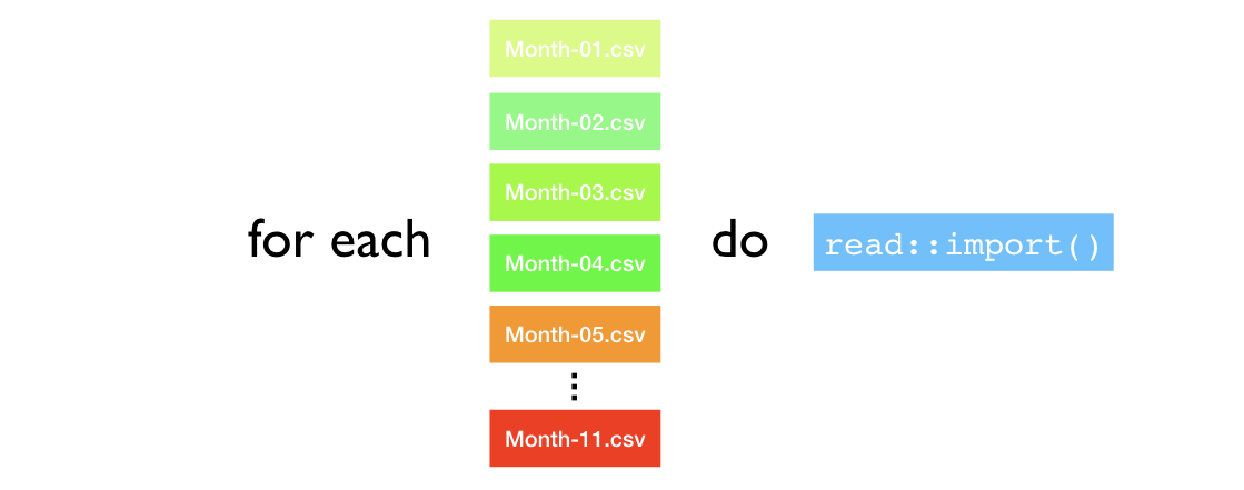
Figure 23.1: Intent of iteration statements.

Functional programming turns this idea into a function which, as we’ll see in later examples, can help to make iteration more efficient, strict, and explicit!

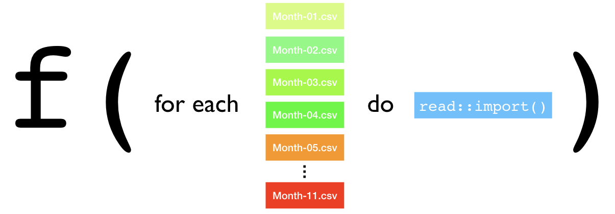
Figure 23.2: Functional programming view of iteration statements.

The purrr package provides functional programming tools that:

• for each element of x
• apply function f and
• provide consistent output

The most common use of purrr functions focus around the family of map() functions. The family of map functions provided by purrr consist of vectorized functions which minimize your need to explicitly create loops. The initial functions we’ll explore include

• map() outputs a list.
• map_lgl() outputs a logical vector.
• map_int() outputs an integer vector.
• map_dbl() outputs a double vector.
• map_chr() outputs a character vector.
• map_df() outputs a data frame.

These functions all behave in a similar manner - they each take a vector as input, applies a function to each piece, and then returns a new vector that’s the same length as the input. The primary difference is in the object they return.

For example, say we wanted to iterate over the Complete Journey demographics data frame and compute the number of unique values for each column. We could do this with a for loop, which would look like this:

cols <- colnames(completejourney::demographics)
distinct_values <- vector(mode = 'integer', length = length(cols))

for (column in seq_along(cols)) {
   n_dist <- n_distinct(completejourney::demographics[column])
   distinct_values[column] <- n_dist
} 

distinct_values
## [1] 801   6  12   5   3   5   4   4

However, admittedly, this is a bit busy and its tough to see what the primary intent of this code is. Alternatively, we could apply purrr::map, which in this example will iterate over each column of completejourney::demographics and apply the n_distinct function.

# tidyverse automatically loads purrr
library(tidyverse)

completejourney::demographics %>%
   map(n_distinct)
## $household_id
## [1] 801
## 
## $age
## [1] 6
## 
## $income
## [1] 12
## 
## $home_ownership
## [1] 5
## 
## $marital_status
## [1] 3
## 
## $household_size
## [1] 5
## 
## $household_comp
## [1] 4
## 
## $kids_count
## [1] 4

Notice how the above results in a named list. If instead we wanted a vector to be returned we can us map_int:

completejourney::demographics %>%
   map_int(n_distinct)
##   household_id            age         income home_ownership 
##            801              6             12              5 
## marital_status household_size household_comp     kids_count 
##              3              5              4              4

We can apply other map functions to our input as well; we simply need to think about what we expect the output to be and that directs us to use the relevant map function:

# logical output
completejourney::demographics %>% map_lgl(is.factor)
##   household_id            age         income home_ownership 
##          FALSE           TRUE           TRUE           TRUE 
## marital_status household_size household_comp     kids_count 
##           TRUE           TRUE           TRUE           TRUE

# integer output
completejourney::demographics %>% map_int(~ length(unique(.)))
##   household_id            age         income home_ownership 
##            801              6             12              5 
## marital_status household_size household_comp     kids_count 
##              3              5              4              4

Notice the last function applied looks different. The map functions provide a few shortcuts that you can use with the .f argument in order to save a little typing. The syntax for creating an anonymous function in R is quite verbose so purrr provides a convenient shortcut: a one-sided formula where . inside of unique points where the data should be evaluated.

# traditional anonymous function approach
completejourney::demographics %>% map_int(function(x) length(unique(x)))
##   household_id            age         income home_ownership 
##            801              6             12              5 
## marital_status household_size household_comp     kids_count 
##              3              5              4              4

# one-sided formula approach
completejourney::demographics %>% map_int(~ length(unique(.)))
##   household_id            age         income home_ownership 
##            801              6             12              5 
## marital_status household_size household_comp     kids_count 
##              3              5              4              4

This, along with chaining multiple map functions together, can make for very efficient data mining. To provide a toy example, the following uses the diamonds data set provided by ggplot2 and:

1. breaks the data set into separate data frames based on the cut variable,
2. applies a linear regression model to each data frame,
3. extracts the summary of each linear regression model, and
4. computes the \(R^2\) for each model.

Don’t worry, in the next module you’ll learn more about applying statistical models to your data. For now, just work through each line of code to get insight into the input and output of each map step.

diamonds %>% 
   split(.$cut) %>% 
   map(~lm(price ~ carat, data = .)) %>%
   map(summary) %>% 
   map_dbl(~.$r.squared)
##      Fair      Good Very Good   Premium     Ideal 
##   0.73839   0.85095   0.85816   0.85563   0.86709

23.5.1 Knowledge check

With the built-in airquality data set, use the most appropriate map functions to answer these three questions:

1. How many n_distinct values are in each column?
2. Are there any missing values in this data set?
3. What is the standard deviation for each variable?

If you want to get deeper into functional programming with purrr check out Section 21.5 of R for Data Science.

23.6 Exercises

1. Use purrr::map_dfr to import each of the monthly_data/Month-XX.csv data files and combine into one single data frame.
2. Check the current class of each column i.e. (class(df$Account_ID)). Since the time stamp variable has two classes, you can’t condense this down to an atomic vector.
3. How many unique values exist in each column?