3 Lesson 1b: R fundamentals
This lesson serves to introduce you to many of the basics of R to get you comfortable. This includes understanding how to assign and evaluate expressions, performing basic calculator-like activities, the idea of vectorization and packages. Finally, I offer some basic styling guidelines to help you write code that is easier to digest by others.
3.1 Learning objectives
Upon completing this module you will be able to:
- Assign values to variables and evaluate them.
- Perform basic mathematical operations.
- Explain what packages and be able to install and load them.
- Understand and apply basic styling guidelines to your code.
3.2 Assignment & evaluation
3.2.1 Assignment
The first operator you’ll run into is the assignment operator. The assignment operator is used to assign a value. For instance we can assign the value 3 to the variable x using the <- assignment operator.
R is a dynamically typed programming language which means it will
perform the process of verifying and enforcing the constraints of types
at run-time. If you are unfamiliar with dynamically versus
statically-typed languages then do not worry about this detail. Just
realize that dynamically typed languages allow for the simplicity of
running the above command and R automatically inferring that
3 should be a numeric type rather than a character
string.
Interestingly, R actually allows for five assignment operators3:
# leftward assignment
x <- value
x = value
x <<- value

# rightward assignment
value -> x
value ->> x
The original assignment operator in R was <- and has continued to be the preferred among R users. The = assignment operator was added in 2001 primarily because it is the accepted assignment operator in many other languages and beginners to R coming from other languages were so prone to use it. Using = is not wrong, just realize that most R programmers prefer to keep = reserved for argument association and use <- for assignment.
The operators <<- is normally only used in functions or looping constructs which we will not get into the details. And the rightward assignment operators perform the same as their leftward counterparts, they just assign the value in an opposite direction.
Overwhelmed yet? Don’t be. This is just meant to show you that there are options and you will likely come across them sooner or later. My suggestion is to stick with the tried, true, and idiomatic <- operator. This is the most conventional assignment operator used and is what you will find in all the base R source code…which means it should be good enough for you.
3.2.2 Evaluation
We can then evaluate the variable by simply typing x at the command line which will return the value of x. Note that prior to the value returned you’ll see ## [1] in the console. This simply implies that the output returned is the first output. Note that you can type any comments in your code by preceding the comment with the hash tag (#) symbol. Any values, symbols, and texts following # will not be evaluated.
3.3 R as a calculator
3.3.1 Basic Arithmetic
At its most basic function R can be used as a calculator. When applying basic arithmetic, the PEMDAS order of operations applies: parentheses first followed by exponentiation, multiplication and division, and finally addition and subtraction.
8 + 9 / 5 ^ 2
## [1] 8.36

8 + 9 / (5 ^ 2)
## [1] 8.36

8 + (9 / 5) ^ 2
## [1] 11.24

(8 + 9) / 5 ^ 2
## [1] 0.68
By default R will display seven digits but this can be changed using options() as previously outlined.
Also, large numbers will be expressed in scientific notation which can also be adjusted using options().
Note that the largest number of digits that can be displayed is 22. Requesting any larger number of digits will result in an error message.
pi
## [1] 3.141592654

options(digits = 22)
pi
## [1] 3.141592653589793115998

options(digits = 23)
## Error in options(digits = 23): invalid 'digits' parameter, allowed 1...22
pi
## [1] 3.141592653589793115998
We can also perform integer divide (%/%) and modulo (%%) functions. The integer divide function will give the integer part of a fraction while the modulo will provide the remainder.
3.3.2 Miscellaneous Mathematical Functions
There are many built-in functions to be aware of. These include but are not limited to the following. Go ahead and run this code in your console.
3.3.3 Infinite, and NaN Numbers
When performing undefined calculations, R will produce Inf (infinity) and NaN (not a number) outputs. These can easily pop up in regular data wrangling tasks and later modules will discuss how to work with these types of outputs along with missing values.
# infinity
1 / 0
## [1] Inf

# infinity minus infinity
Inf - Inf
## [1] NaN

# negative infinity
-1 / 0
## [1] -Inf

# not a number
0 / 0
## [1] NaN

# square root of -9
sqrt(-9)
## Warning in sqrt(-9): NaNs produced
## [1] NaN
3.3.4 Knowledge check
-
Assign the values 1000, 5, and 0.05 to variables
D,K, andhrespectively. - Compute \(2 \times D \times K\).
- Compute \(\frac{2 \times D \times K}{h}\).
-
Now put this together to compute the Economic Order Quantity, which
is \(\sqrt{\frac{2 \times D \times
K}{h}}\). Save the output as
Q.
3.4 Working with packages
In R, the fundamental unit of shareable code is the package. A package bundles together code, data, documentation, and tests and provides an easy method to share with others (Wickham 2015). As of April 2022 there were nearly 19,000 packages available on CRAN, 2,000 on Bioconductor, and countless more available through GitHub. This huge variety of packages is one of the reasons that R is so successful: chances are that someone has already solved a problem that you’re working on, and you can benefit from their work by downloading and using their package.
3.4.1 Installing Packages
The most common place to get packages is from CRAN. To install packages from CRAN you use install.packages("packagename"). For instance, if you want to install the ggplot2 package, which is a very popular visualization package you would type the following in the console:
As previously stated, packages are also available through Bioconductor and GitHub. Bioconductor provides R packages primarily for genomic data analyses and packages on GitHub are usually under development but have not gone through all the checks and balances to be loaded onto CRAN (aka download and use these packages at your discretion). You can learn how to install Bioconductor packages here and GitHub packages here.
3.4.2 Loading Packages
Once the package is downloaded to your computer you can access the functions and resources provided by the package in two different ways:
# load the package to use in the current R session
library(packagename)

# use a particular function within a package without loading the package
packagename::functionname
For instance, if you want to have full access to the dplyr package you would use library(dplyr); however, if you just wanted to use the filter() function which is provided by the dplyr package without fully loading dplyr you can use dplyr::filter(...)4.
3.4.3 Getting Help on Packages
For more direct help on packages that are installed on your computer you can use the help and vignette functions. Here we can get help on the ggplot2 package with the following:
help(package = "ggplot2")      # provides details regarding contents of a package
vignette(package = "ggplot2")  # list vignettes available for a specific package
vignette("ggplot2-specs")      # view specific vignette
vignette()                     # view all vignettes on your computer
Note that some packages will have multiple vignettes. For instance vignette(package = "grid") will list the 13 vignettes available for the grid package. To access one of the specific vignettes you simply use vignette("vignettename").
3.4.4 Useful Packages
There are thousands of helpful R packages for you to use, but navigating them all can be a challenge. To help you out, RStudio compiled a guide to some of the best packages for loading, manipulating, visualizing, analyzing, and reporting data. In addition, their list captures packages that specialize in spatial data, time series and financial data, increasing spead and performance, and developing your own R packages.
3.4.5 Knowledge check
- Install the completejourney package.
- Load the completejourney package.
- Access the help documentation for the completejourney package.
- Check out the vignette(s) for completejourney.
-
Call the
get_transactions()function provided by completejourney and save the output to atransactionsvariable (note that this takes a little time as you are trying to download 1.5 million transactions!).
3.4.6 Tidyverse
The tidyverse is an opinionated collection of R packages designed for data science. All packages share an underlying design philosophy, grammar, and data structures; and this group of packages has become extremely popular and common across the data science community. You will learn about many of these packages throughout this course.
Take a little time to familiarize yourself with the Tidyverse. Not only will you find high-level descriptions of the different tidyverse packages but you will also find a lot of educational content that you can and should take advantage of!
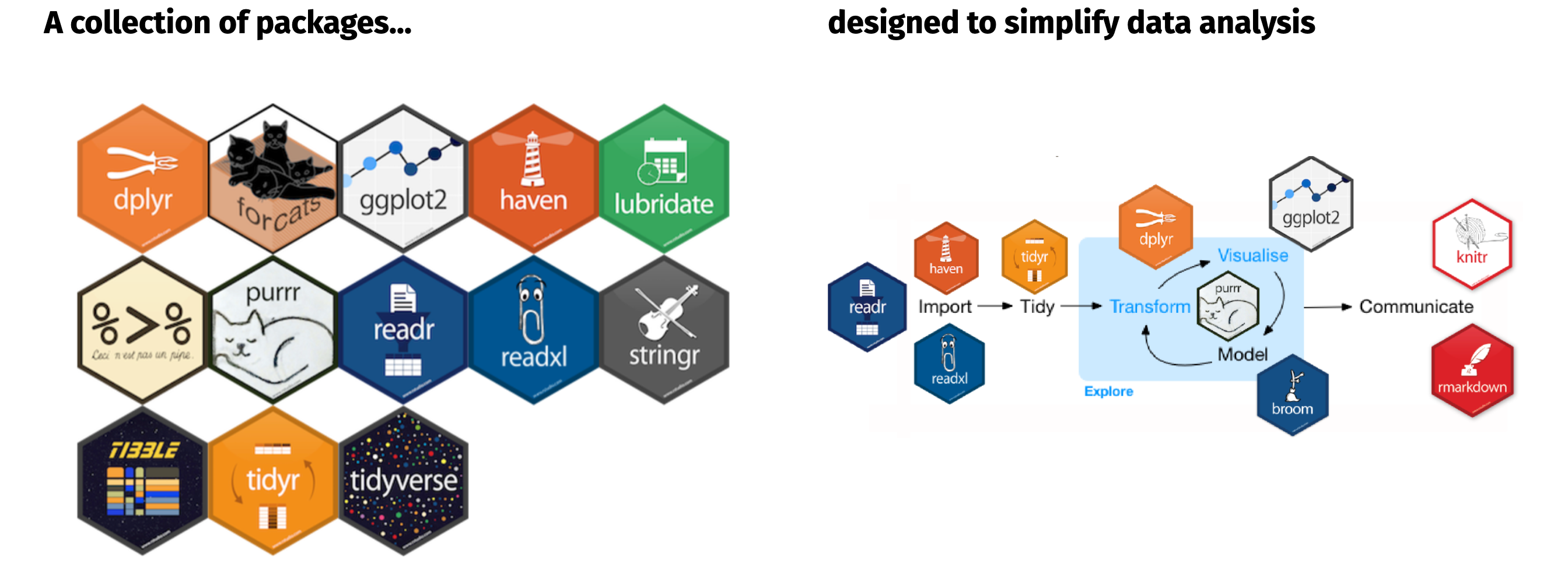
Figure 3.1: Tidyverse is a collection of packages designed to simplify many tasks throughout the data analysis process.
Let’s go ahead and install the tidyverse package, which will actually install a bunch of other packages for us.
The single line of code above 👆…
is equivalent to running the 29 lines of code below 👇!
install.packages("ggplot2")
install.packages("tibble")
install.packages("tidyr")
install.packages("readr")
install.packages("purrr")
install.packages("dplyr")
install.packages("stringr")
install.packages("forcats")
install.packages("cli")
install.packages("crayon")
install.packages("dbplyr")
install.packages("dtplyr")
install.packages("googledrive")
install.packages("googlesheets4")
install.packages("haven")
install.packages("hms")
install.packages("httr")
install.packages("jsonlite")
install.packages("lubridate")
install.packages("magrittr")
install.packages("modelr")
install.packages("pillar")
install.packages("readxl")
install.packages("reprex")
install.packages("rlang")
install.packages("rstudioapi")
install.packages("rvest")
install.packages("xml2")
If we load the tidyverse package we will see that it loads 8 packages for us: ggplot2_, tibble, tidyr, readr, purrr, dplyr, stringr, and forcats. These are packages that we will tend to use in almost any data analysis project.
library(tidyverse)
## ── Attaching core tidyverse packages ─────────────── tidyverse 2.0.0 ──
## ✔ dplyr     1.1.4     ✔ readr     2.1.5
## ✔ forcats   1.0.0     ✔ stringr   1.5.1
## ✔ ggplot2   3.5.1     ✔ tibble    3.2.1
## ✔ lubridate 1.9.3     ✔ tidyr     1.3.1
## ✔ purrr     1.0.2
## ── Conflicts ───────────────────────────────── tidyverse_conflicts() ──
## ✖ dplyr::filter() masks stats::filter()
## ✖ dplyr::lag()    masks stats::lag()
## ℹ Use the conflicted package (<http://conflicted.r-lib.org/>) to force all conflicts to become errors
The single line of code above 👆…
is equivalent to running the 8 lines of code below 👇!
library(ggplot2)
library(tibble)
library(tidyr)
library(readr)
library(purrr)
library(dplyr)
library(stringr)
library(forcats)
3.5 Style guide
“Good coding style is like using correct punctuation. You can manage without it, but it sure makes things easier to read.” - Hadley Wickham
As a medium of communication, its important to realize that the readability of code does in fact make a difference. Well styled code has many benefits to include making it easy to i) read, ii) extend, and iii) debug. Unfortunately, R does not come with official guidelines for code styling but such is an inconvenient truth of most open source software. However, this should not lead you to believe there is no style to be followed and over time implicit guidelines for proper code styling have been documented.
What follows are a few of the basic guidelines from the tidyverse style guide. These suggestions will help you get started with good styling suggestions as you begin this book but as you progress you should leverage the far more detailed tidyverse style guide along with useful packages such as lintr and styler to help enforce good code syntax on yourself.
3.5.1 Notation and Naming
File names should be meaningful and end with a .R extension.
If files need to be run in sequence, prefix them with numbers:
In R, naming conventions for variables and functions are famously muddled. They include the following:
namingconvention        # all lower case; no separator
naming.convention       # period separator
naming_convention       # underscore separator (aka snake case)
namingConvention        # lower camel case
NamingConvention        # upper camel case
Historically, there has been no clearly preferred approach with multiple naming styles sometimes used within a single package. Bottom line, your naming convention will be driven by your preference but the ultimate goal should be consistency.
Vast majority of the R community uses lowercase with an underscore (“_“) to separate words within a variable/function name (‘snake_case’). Furthermore, variable names should be nouns and function names should be verbs to help distinguish their purpose. Also, refrain from using existing names of functions (i.e. mean, sum, true).
3.5.2 Organization
Organization of your code is also important. There’s nothing like trying to decipher 500 lines of code that has no organization. The easiest way to achieve organization is to comment your code. When you have large sections within your script you should separate them to make it obvious of the distinct purpose of the code.
# Download Data -------------------------------------------------------------------
lines of code here

# Preprocess Data -----------------------------------------------------------------
lines of code here

# Exploratory Analysis ------------------------------------------------------------
lines of code here
You can easily add these section breaks within RStudio wth Cmd+Shift+R.
Then comments for specific lines of code can be done as follows:
code_1  # short comments can be placed to the right of code
code_2  # blah
code_3  # blah

# or comments can be placed above a line of code
code_4

# Or extremely long lines of commentary that go beyond the suggested 80
# characters per line can be broken up into multiple lines. Just don't forget
# to use the hash on each.
code_5
You can easily comment or uncomment lines by highlighting the line and then pressing Cmd+Shift+C.
3.5.3 Syntax
The maximum number of characters on a single line of code should be 80 or less. If you are using RStudio you can have a margin displayed so you know when you need to break to a new line5. Also, when indenting your code use two spaces rather than using tabs. The only exception is if a line break occurs inside parentheses. In this case it is common to do either of the following:
# option 1
super_long_name <- seq(ymd_hm("2015-1-1 0:00"),
                       ymd_hm("2015-1-1 12:00"),
                       by = "hour")

# option 2
super_long_name <- seq(
  ymd_hm("2015-1-1 0:00"),
  ymd_hm("2015-1-1 12:00"),
  by = "hour"
)
Proper spacing within your code also helps with readability. Place spaces around all infix operators (=, +, -, <-, etc.). The same rule applies when using = in function calls. Always put a space after a comma, and never before.
# Good
average <- mean(feet / 12 + inches, na.rm = TRUE)

# Bad
average<-mean(feet/12+inches,na.rm=TRUE)
There’s a small exception to this rule: :, :: and ::: don’t need spaces around them.
It is important to think about style when communicating any form of language. Writing code is no exception and is especially important if your code will be read by others. Following these basic style guides will get you on the right track for writing code that can be easily communicated to others.
3.5.4 Knowledge check
- Review chapters 1 & 2 in the Tidyverse Style Guide.
-
Go back through the script you’ve been writing to execute the
exercises in this module and make sure
- your naming conventions are consistent,
- your code is nicely organized and annotated,
- your syntax includes proper spacing.
3.6 Exercises
-
Say you have a 12” pizza. Compute the area of the pizza and assign
that value to the variable
area. Now say thecostof the pizza was $8. Compute the cost per square inch and assign that value to a variableppsi. -
Based on the style guide section rename the
ppsivariable in question 1 to be more meaningful. - If you did not already do so, install the tidyverse package.
- How many vignettes does the dplyr package have?
- Where can you go to learn more about the tidyverse packages?
- When you load the tidyverse packages what other packages is it automatically loading for you?
- Using the resource in #5, explain at a high-level what the packages in #6 do.