14 Lesson 4a: Relational data
It’s rare that a data analysis involves only a single table of data. Typically you have many tables of data, and you must combine them to answer the questions that you’re interested in. Collectively, multiple tables of data are called relational data because its the relations, not just the individual data sets, that are important.
To work with relational data you need join operations that work with pairs of tables. There are two families of verbs designed to work with relational data:
- Mutating joins: add new variables to one data frame by matching observations in another.
- Filter joins: filter observations from one data frame based on whether or not they match an observation in the other table.
In this lesson, we are going to look at different ways to apply mutating and filtering joins to relational data sets.
14.1 Learning objectives
By the end of this lesson you’ll be able to:
- Use various mutating joins to combine variables from two tables.
- Use filtering joins to filter one data set based on observations in another data set.
14.2 Prerequisites
Load the dplyr package to provide you access to the join functions we’ll cover in this lesson.
To illustrate various joining tasks we will use two very simple data frames x & y. The colored column represents the “key” variable: these are used to match the rows between the tables. We’ll talk more about keys in a second. The grey column represents the “value” column that is carried along for the ride.
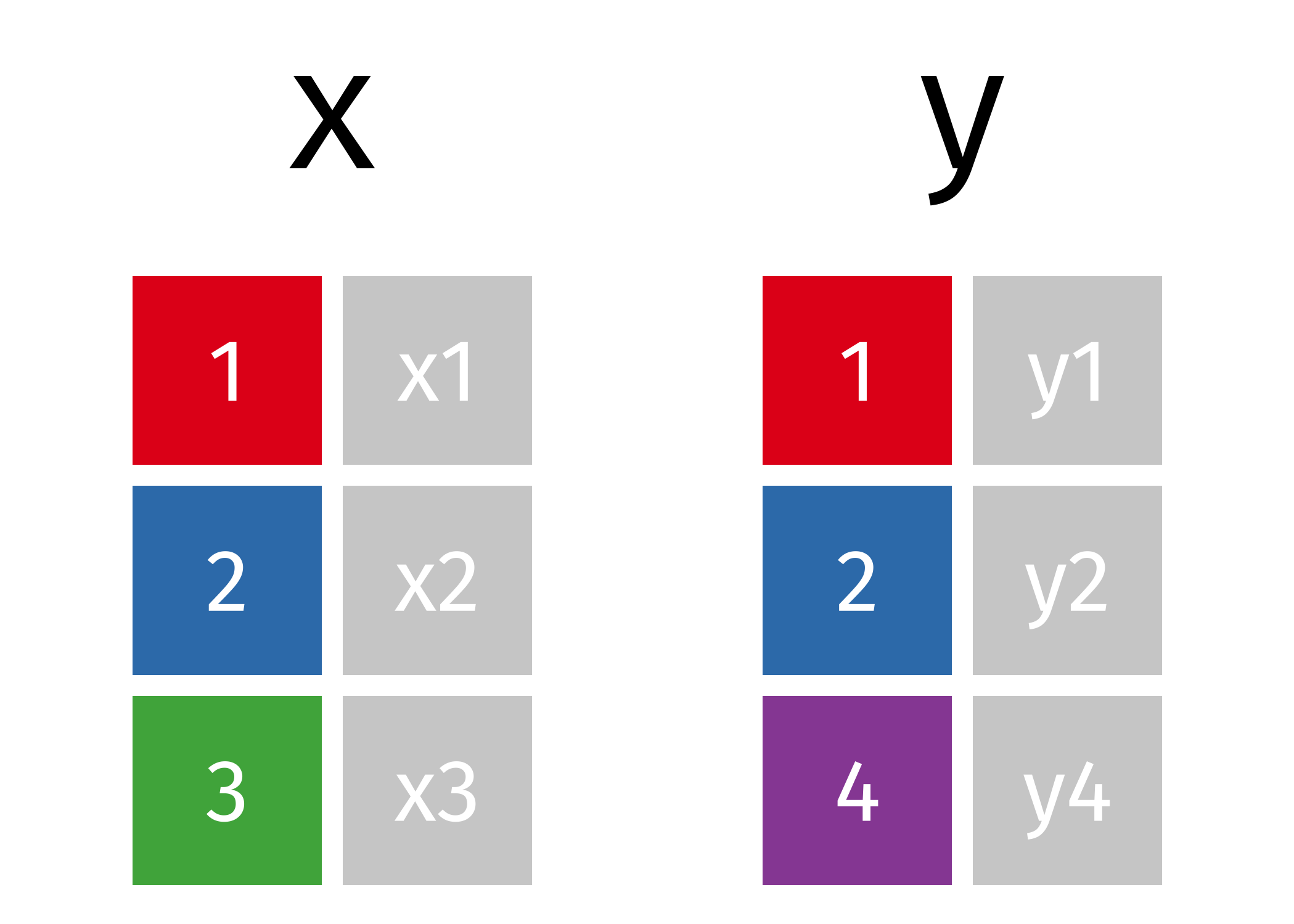
Figure 14.1: Two simple data frames.
x <- tribble(
  ~id, ~val_x,
     1, "x1",
     2, "x2",
     3, "x3"
)
y <- tribble(
  ~id, ~val_y,
     1, "y1",
     2, "y2",
     4, "y3"
)
However, we will also build upon the simple examples by using various data sets from the completejourney library:
Take some time to read about the various data sets available via completejourney.
- What different data sets are available and what do they represent?
- What are the common variables between each table?
14.3 Keys
The variables used to connect two tables are called keys. A key is a variable (or set of variables) that uniquely identifies an observation. There are two primary types of keys we’ll consider in this lesson:
- A primary key uniquely identifies an observation in its own table
- A foreign key uniquely identifies an observation in another table
Variables can be both a primary key and a foreign key. For example, within the transactions data household_id is a primary key to represent a household identifier for each transaction. household_id is also a foreign key in the demographics data set where it can be used to align household demographics to each transaction.
A primary key and the corresponding foreign key in another table form a relation. Relations are typically one-to-many. For example, each transaction has one household, but each household has many transactions. In other data, you’ll occasionally see a 1-to-1 relationship.
When data is cleaned appropriately the keys used to match two tables will be commonly named. For example, the variable that can link our x and y data sets is named id:
We can easily see this by looking at the data but when working with larger data sets this becomes more appropriate than just viewing the data.
Although it is preferred, keys do not need to have the same name in
both tables. For example, our household identifier could be named
household_id in the transaction data but be
hshd_id in the demographics table. The names would be
different but they represent the same information.
14.3.1 Knowledge check
Using the completejourney data, programmatically identify the common key(s) that between:
-
transactions_sampleandproductstables. -
demographicsandcampaignstables. -
campaignsandcampaign_descriptionstables. -
Is there a common key between
transactions_sampleandcoupon_redemptions? Does this mean we can or cannot join these two data sets?
14.4 Mutating joins
Often we have separate data frames that can have common and differing variables for similar observations and we wish to join these data frames together. A mutating join allows you to combine variables from two tables. It first matches observations by their keys, then copies across variables from one table to the other.
dplyr offers multiple mutating join functions (xxx_join()) that provide alternative ways to join two data frames:
inner_join(): keeps only observations inxthat match iny.left_join(): keeps all observations inxand adds available information fromy.right_join(): keeps all observations inyand adds available information fromx.full_join(): keeps all observations in bothxandy.
Let’s explore each of these a little more closely.
14.4.1 Inner join
The simplest type of join is the inner join. An inner join matches pairs of observations whenever their keys are equal. Consequently, the output of an inner join is all rows from x where there are matching values in y, and all columns from x and y.
An inner join is the most restrictive of the joins - it returns only rows with matches across both data frames.
The following provides a nice illustration:
).](images/inner-join.gif)
Figure 14.2: Inner join (source).
14.4.2 Outer joins
An inner join keeps observations that appear in both tables. However, we often want to retain all observations in at least one of the tables. Consequently, we can apply various outer joins to retain observations that appear in at least one of the tables. There are three types of outer joins:
- A left join keeps all observations in
x. - A right join keeps all observations in
y. - A full join keeps all observations in
xandy.
14.4.2.1 Left join
With a left join we retain all observations from x, and we add columns y. Rows in x where there is no matching key value in y will have NA values in the new columns.
).](images/left-join.gif)
Figure 14.3: Left join (source).
14.4.2.2 Right join
A right join is just a flipped left join where we retain all observations from y, and we add columns x. Similar to a left join, rows in y where there is no matching key value in x will have NA values in the new columns.
Should I use a right join, or a left join? To answer this, ask yourself “which data frame should retain all of its rows?” - and use this one as the baseline. A left join keep all the rows in the first data frame written in the command, whereas a right join keeps all the rows in the second data frame.
).](images/right-join.gif)
Figure 14.4: Right join (source).
14.4.2.3 Full join
We can also perform a full join where we keep all observations in x and y. This join will match observations where the key variable(s) have matching information in both tables and then fill in non-matching values as NA.
A full join is the most inclusive of the joins - it returns all rows from both data frames.
).](images/full-join.gif)
Figure 14.5: Full join (source).
14.4.3 Differing keys
So far, the keys we’ve used to join two data frames have had the same name. This was encoded by using by = "id". However, this is not a requirement. In fact, if we exclude the by argument then our xxx_join() functions will identify all common variable names in both tables and join by those. When this happens we get a message:
x %>% inner_join(y)
## Joining with `by = join_by(id)`
## # A tibble: 2 × 3
##      id val_x val_y
##   <dbl> <chr> <chr>
## 1     1 x1    y1
## 2     2 x2    y2
But what happens we our common key variable is named differently in each data frame?
a <- tribble(
  ~id_1, ~val_a,
      1, "x1",
      2, "x2",
      3, "x3"
)
b <- tribble(
  ~id_2, ~val_b,
      1, "y1",
      2, "y2",
      4, "y3"
)
In this case, since our common key variable has different names in each table (id_1 in a and id_2 in b), our inner join function doesn’t know how to join these two data frames.
a %>% inner_join(b)
## Error in `inner_join()`:
## ! `by` must be supplied when `x` and `y` have no common
##   variables.
## ℹ Use `cross_join()` to perform a cross-join.
When this happens, we can explicitly tell our join function to use two unique key names as a common key:
14.4.4 Bigger example
So far we’ve used small simple examples to illustrate the differences between joins. Now let’s use our completejourney data to look at some larger examples.
Say we wanted to add product information (via products) to each transaction (transaction_sample); however, we want to retain all transactions. This would suggest a left join so we can keep all transaction observations but simply add product information where possible to each transaction.
First, let’s get the common key:
This aligns to the data dictionary so we can trust this is the accurate common key. We can now perform a left join using product_id as the common key:
Like mutate(), the join functions add variables to the
right, so if you have a lot of variables already, the new variables
won’t get printed out. You can also use View() on the
output to show the resulting table in a spreadsheet like view.
transactions_sample %>%
   left_join(products, by = "product_id")
## # A tibble: 75,000 × 17
##    household_id store_id basket_id   product_id quantity sales_value
##    <chr>        <chr>    <chr>       <chr>         <dbl>       <dbl>
##  1 2261         309      31625220889 940996            1        3.86
##  2 2131         368      32053127496 873902            1        1.59
##  3 511          316      32445856036 847901            1        1
##  4 400          388      31932241118 13094913          2       11.9
##  5 918          340      32074655895 1085604           1        1.29
##  6 718          324      32614612029 883203            1        2.5
##  7 868          323      32074722463 9884484           1        3.49
##  8 1688         450      34850403304 1028715           1        2
##  9 467          31782    31280745102 896613            2        6.55
## 10 1947         32004    32744181707 978497            1        3.99
## # ℹ 74,990 more rows
## # ℹ 11 more variables: retail_disc <dbl>, coupon_disc <dbl>,
## #   coupon_match_disc <dbl>, week <int>, transaction_timestamp <dttm>,
## #   manufacturer_id <chr>, department <chr>, brand <fct>,
## #   product_category <chr>, product_type <chr>, package_size <chr>
This has now added product information to each transaction. Consequently, if we wanted to get the total sales across the meat department but summarized at the product_category level so that we can identify which products generate the greatest sales we could follow this joining procedure with additional skills we learned in previous lessons:
transactions_sample %>%
   left_join(products, by = "product_id") %>%
   filter(department == 'MEAT') %>%
   group_by(product_category) %>%
   summarize(total_spend = sum(`sales_value`)) %>%
   arrange(desc(total_spend))
## # A tibble: 9 × 2
##   product_category        total_spend
##   <chr>                         <dbl>
## 1 BEEF                        8800.
## 2 CHICKEN                     2540.
## 3 PORK                        2527.
## 4 SMOKED MEATS                 784.
## 5 TURKEY                       625.
## 6 EXOTIC GAME/FOWL              61
## 7 LAMB                          34.7
## 8 MEAT - MISC                    4.63
## 9 RW FRESH PROCESSED MEAT        1.69
14.4.5 Knowledge check
-
Join the
transactions_sampleanddemographicsdata so that you have household demographics for each transaction. Now compute the total sales byagecategory to identify which age group generates the most sales. -
Use successive joins to join
transactions_samplewithcouponsand then withcoupon_redemptions. Use the proper join that will only retain those transactions that have coupon and coupon redemption data.
14.5 Filtering joins
In certain situations, we may want to filter one data set based on observations in another data set but not add new information. Whereas mutating joins are for the purpose of adding columns and rows from one data set to another, filtering joins are for the purpose of filtering.
Filtering joins include:
semi_join(): keeps all observations inxthat have a match iny.anti_join(): drops all observations inxthat have a match iny.
14.5.1 Semi join
A semi-join keeps all observations in the baseline data frame that have a match in the secondary data frame (but does not add new columns nor duplicate any rows for multiple matches).
).](images/semi-join.gif)
Figure 14.6: Semi join (source).
14.5.2 Anti join
The anti join is another “filtering join” that returns rows in the baseline data frame that do not have a match in the secondary data frame.
Common scenarios for an anti-join include identifying records not present in another data frame, troubleshooting spelling in a join (reviewing records that should have matched), and examining records that were excluded after another join.
).](images/anti-join.gif)
Figure 14.7: Anti join (source).
14.5.3 Bigger example
We can use the completejourney data to highlight the purpose behind filtering joins. In our transactions_sample we have a total of 75,000 transactions.
Now say our manager came to us and asked – “of all our transactions, how many of them are related to households that we have demographic information on?” To answer this question we would use a semi-join, which shows that 42,199 (56%) of our transactions are for customers that we have demographics on.
transactions_sample %>%
   semi_join(demographics, by = "household_id") %>%
   tally()
## # A tibble: 1 × 1
##       n
##   <int>
## 1 42199
Now, what if our manager asked us the same question but with a slightly different angle – “of all our transactions, how many of them are by customers that we don’t have demographic information on?” To answer this question we would use an anti-join, which shows that 32,801 (44%) of our transactions are for customers that we do not have demographics on.
14.5.4 Knowledge check
-
Using the
productsandtransactions_sampledata, how many products have and have not sold? In other words, of all the products we have in our inventory, how many have a been involved in a transaction? How many have not been involved in a transaction? -
Using the
demographicsandtransactions_sampledata, identify whichincomelevel buys the mostquantityof goods.
14.6 Exercises
-
Get demographic information for all households that have total sales
(
sales_value) of $100 or more. - Of the households that have total sales of $100 or more, how many of these customers do we not have demographic information on?
-
Using the
promotions_sampleandtransactions_sampledata, compute the total sales for all products that were in a display in the front of the store (display_location–> 1).