8 Lesson 2c: Importing data
The first step to any data analysis process is to get the data. Data can come from many sources but two of the most common include delimited and Excel files. This section covers how to import data from these common files; plus we cover other important topics such as understanding file paths, connecting to SQL databases, and to load data from saved R object files.
8.1 Learning objectives
Upon completing this module you will be able to:
- Describe how imported data affects computer memory.
- Import tabular data with R.
- Assess some basic attributes of your imported data.
- Import alternative data files such as SQL tables and Rdata files.
8.2 Data & memory
R stores its data in memory - this makes it relatively quickly accessible but can cause size limitations in certain fields. In this class we will mainly work with small to moderate data sets, which means we should not run into any space limitations.
R does provide tooling that allows you to work with big data via distributed data (i.e. sparklyr) and relational databrases (i.e. SQL).
R memory is session-specific, so quitting R (i.e. shutting down RStudio) removes the data from memory. A general way to conceptualize data import into and use within R:
- Data sits in on the computer/server - this is frequently called “disk”
- R code can be used to copy a data file from disk to the R session’s memory
- R data then sits within R’s memory ready to be used by other R code
Here is a visualization of this process:
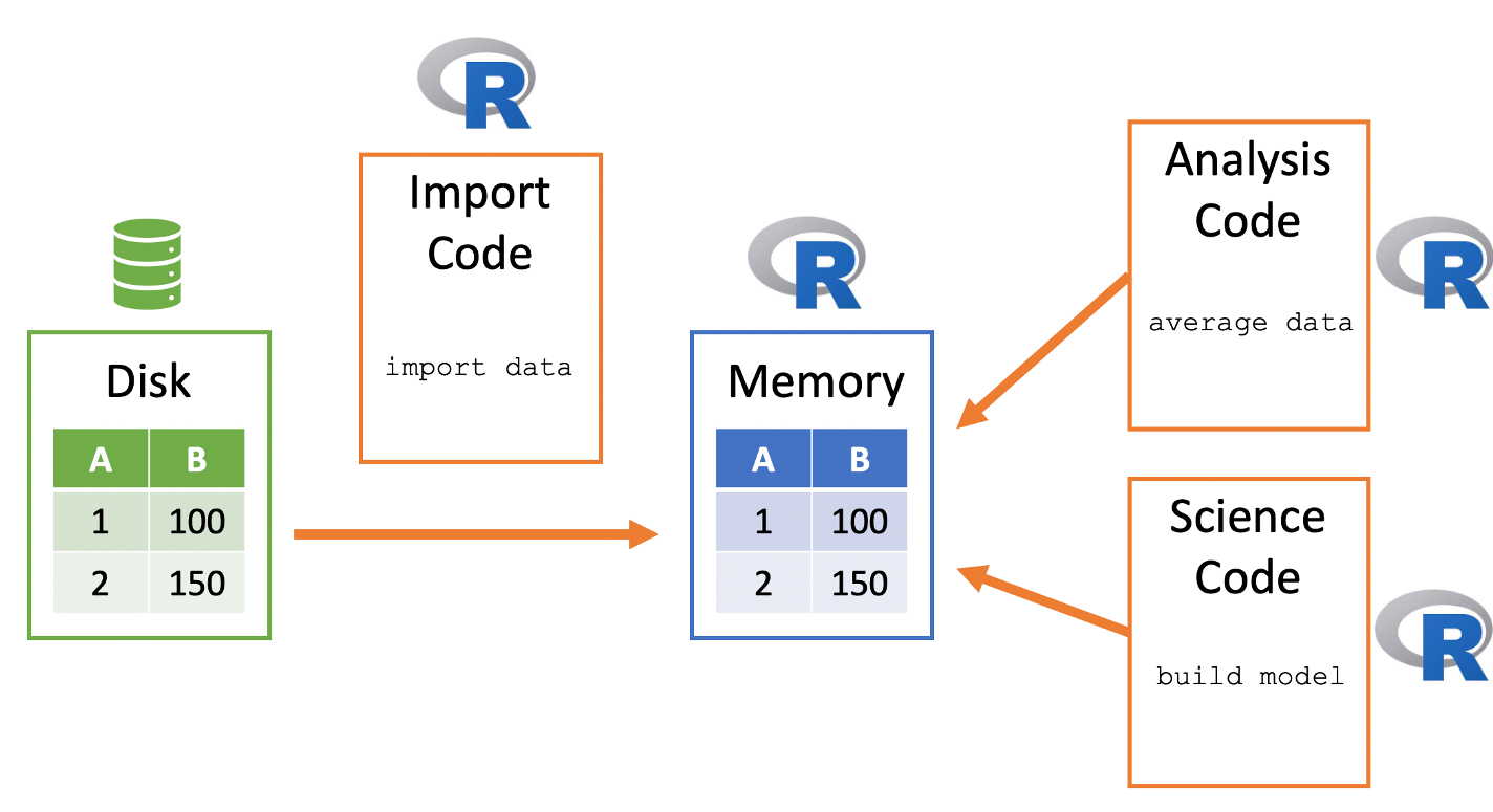
Figure 8.1: Conceptualizing how R imports data.
8.3 Delimited files
Text files are a popular way to hold and exchange tabular data as almost any data application supports exporting data to the CSV (or other text file) format. Text file formats use delimiters to separate the different elements in a line, and each line of data is in its own line in the text file. Therefore, importing different kinds of text files can follow a fairly consistent process once you’ve identified the delimiter.
There are three main groups of functions that we can use to read in text files:
- Base R functions
- *readr** package functions
- *vroom** package functions
Here, we’ll focus on the middle one.
All three functions will import a tabular delimited file (.csv, .tsv,
.txt, etc.) and convert it to a data frame in R, but each has subtle
differences. You can read why we favor readr and
vroom over the base R importing functions
(i.e. read.csv()) here.
We will not cover the vroom package but it is good to know about as it can be extremely fast for very large data sets. Read more about vroom here.
The following will import a data set describing the sale of individual residential property in Ames, Iowa from 2006 to 2010 (source).
You can download this data from the supplemental files in Canvas.
library(readr)

ames <- read_csv('data/ames_raw.csv')
## Rows: 2930 Columns: 82
## ── Column specification ───────────────────────────────────────────────
## Delimiter: ","
## chr (45): PID, MS SubClass, MS Zoning, Street, Alley, Lot Shape, La...
## dbl (37): Order, Lot Frontage, Lot Area, Overall Qual, Overall Cond...
##
## ℹ Use `spec()` to retrieve the full column specification for this data.
## ℹ Specify the column types or set `show_col_types = FALSE` to quiet this message.
We can look at it in our notebook or console and we see that it is displayed in a well-organized, concise manner. More on this in a second.
ames
## # A tibble: 2,930 × 82
##    Order PID        `MS SubClass` `MS Zoning` `Lot Frontage` `Lot Area`
##    <dbl> <chr>      <chr>         <chr>                <dbl>      <dbl>
##  1     1 0526301100 020           RL                     141      31770
##  2     2 0526350040 020           RH                      80      11622
##  3     3 0526351010 020           RL                      81      14267
##  4     4 0526353030 020           RL                      93      11160
##  5     5 0527105010 060           RL                      74      13830
##  6     6 0527105030 060           RL                      78       9978
##  7     7 0527127150 120           RL                      41       4920
##  8     8 0527145080 120           RL                      43       5005
##  9     9 0527146030 120           RL                      39       5389
## 10    10 0527162130 060           RL                      60       7500
## # ℹ 2,920 more rows
## # ℹ 76 more variables: Street <chr>, Alley <chr>, `Lot Shape` <chr>,
## #   `Land Contour` <chr>, Utilities <chr>, `Lot Config` <chr>,
## #   `Land Slope` <chr>, Neighborhood <chr>, `Condition 1` <chr>,
## #   `Condition 2` <chr>, `Bldg Type` <chr>, `House Style` <chr>,
## #   `Overall Qual` <dbl>, `Overall Cond` <dbl>, `Year Built` <dbl>,
## #   `Year Remod/Add` <dbl>, `Roof Style` <chr>, `Roof Matl` <chr>, …
If we check the class of our object we do see that it is a data.frame; however, we also see some additional information. That’s because this is a special kind of data frame known as a tibble.
8.3.1 Tibbles
Tibbles are data frames, but they tweak some older behaviors of data frames to make life a little easier. There are two main differences in the usage of a tibble vs. a classic data frame: printing and subsetting.
Tibbles have a refined print method that shows only the first 10 rows, and all the columns that fit on your screen. This makes it much easier to work with large data. We can see this difference with the following:
# printed output of a tibble
ames
## # A tibble: 2,930 × 82
##    Order PID        `MS SubClass` `MS Zoning` `Lot Frontage` `Lot Area`
##    <dbl> <chr>      <chr>         <chr>                <dbl>      <dbl>
##  1     1 0526301100 020           RL                     141      31770
##  2     2 0526350040 020           RH                      80      11622
##  3     3 0526351010 020           RL                      81      14267
##  4     4 0526353030 020           RL                      93      11160
##  5     5 0527105010 060           RL                      74      13830
##  6     6 0527105030 060           RL                      78       9978
##  7     7 0527127150 120           RL                      41       4920
##  8     8 0527145080 120           RL                      43       5005
##  9     9 0527146030 120           RL                      39       5389
## 10    10 0527162130 060           RL                      60       7500
## # ℹ 2,920 more rows
## # ℹ 76 more variables: Street <chr>, Alley <chr>, `Lot Shape` <chr>,
## #   `Land Contour` <chr>, Utilities <chr>, `Lot Config` <chr>,
## #   `Land Slope` <chr>, Neighborhood <chr>, `Condition 1` <chr>,
## #   `Condition 2` <chr>, `Bldg Type` <chr>, `House Style` <chr>,
## #   `Overall Qual` <dbl>, `Overall Cond` <dbl>, `Year Built` <dbl>,
## #   `Year Remod/Add` <dbl>, `Roof Style` <chr>, `Roof Matl` <chr>, …
# printed output of a regular data frame
as.data.frame(ames)
## Order PID MS SubClass MS Zoning Lot Frontage Lot Area Street
## 1 1 0526301100 020 RL 141 31770 Pave
## 2 2 0526350040 020 RH 80 11622 Pave
## 3 3 0526351010 020 RL 81 14267 Pave
## 4 4 0526353030 020 RL 93 11160 Pave
## 5 5 0527105010 060 RL 74 13830 Pave
## 6 6 0527105030 060 RL 78 9978 Pave
## 7 7 0527127150 120 RL 41 4920 Pave
## 8 8 0527145080 120 RL 43 5005 Pave
## 9 9 0527146030 120 RL 39 5389 Pave
## 10 10 0527162130 060 RL 60 7500 Pave
## 11 11 0527163010 060 RL 75 10000 Pave
## 12 12 0527165230 020 RL NA 7980 Pave
## Alley Lot Shape Land Contour Utilities Lot Config Land Slope
## 1 <NA> IR1 Lvl AllPub Corner Gtl
## 2 <NA> Reg Lvl AllPub Inside Gtl
## 3 <NA> IR1 Lvl AllPub Corner Gtl
## 4 <NA> Reg Lvl AllPub Corner Gtl
## 5 <NA> IR1 Lvl AllPub Inside Gtl
## 6 <NA> IR1 Lvl AllPub Inside Gtl
## 7 <NA> Reg Lvl AllPub Inside Gtl
## 8 <NA> IR1 HLS AllPub Inside Gtl
## 9 <NA> IR1 Lvl AllPub Inside Gtl
## 10 <NA> Reg Lvl AllPub Inside Gtl
## 11 <NA> IR1 Lvl AllPub Corner Gtl
## 12 <NA> IR1 Lvl AllPub Inside Gtl
## Neighborhood Condition 1 Condition 2 Bldg Type House Style
## 1 NAmes Norm Norm 1Fam 1Story
## 2 NAmes Feedr Norm 1Fam 1Story
## 3 NAmes Norm Norm 1Fam 1Story
## 4 NAmes Norm Norm 1Fam 1Story
## 5 Gilbert Norm Norm 1Fam 2Story
## 6 Gilbert Norm Norm 1Fam 2Story
## 7 StoneBr Norm Norm TwnhsE 1Story
## 8 StoneBr Norm Norm TwnhsE 1Story
## 9 StoneBr Norm Norm TwnhsE 1Story
## 10 Gilbert Norm Norm 1Fam 2Story
## 11 Gilbert Norm Norm 1Fam 2Story
## 12 Gilbert Norm Norm 1Fam 1Story
## Overall Qual Overall Cond Year Built Year Remod/Add Roof Style
## 1 6 5 1960 1960 Hip
## 2 5 6 1961 1961 Gable
## 3 6 6 1958 1958 Hip
## 4 7 5 1968 1968 Hip
## 5 5 5 1997 1998 Gable
## 6 6 6 1998 1998 Gable
## 7 8 5 2001 2001 Gable
## 8 8 5 1992 1992 Gable
## 9 8 5 1995 1996 Gable
## 10 7 5 1999 1999 Gable
## 11 6 5 1993 1994 Gable
## 12 6 7 1992 2007 Gable
## Roof Matl Exterior 1st Exterior 2nd Mas Vnr Type Mas Vnr Area
## 1 CompShg BrkFace Plywood Stone 112
## 2 CompShg VinylSd VinylSd None 0
## 3 CompShg Wd Sdng Wd Sdng BrkFace 108
## 4 CompShg BrkFace BrkFace None 0
## 5 CompShg VinylSd VinylSd None 0
## 6 CompShg VinylSd VinylSd BrkFace 20
## 7 CompShg CemntBd CmentBd None 0
## 8 CompShg HdBoard HdBoard None 0
## 9 CompShg CemntBd CmentBd None 0
## 10 CompShg VinylSd VinylSd None 0
## 11 CompShg HdBoard HdBoard None 0
## 12 CompShg HdBoard HdBoard None 0
## Exter Qual Exter Cond Foundation Bsmt Qual Bsmt Cond Bsmt Exposure
## 1 TA TA CBlock TA Gd Gd
## 2 TA TA CBlock TA TA No
## 3 TA TA CBlock TA TA No
## 4 Gd TA CBlock TA TA No
## 5 TA TA PConc Gd TA No
## 6 TA TA PConc TA TA No
## 7 Gd TA PConc Gd TA Mn
## 8 Gd TA PConc Gd TA No
## 9 Gd TA PConc Gd TA No
## 10 TA TA PConc TA TA No
## 11 TA TA PConc Gd TA No
## 12 TA Gd PConc Gd TA No
## BsmtFin Type 1 BsmtFin SF 1 BsmtFin Type 2 BsmtFin SF 2 Bsmt Unf SF
## 1 BLQ 639 Unf 0 441
## 2 Rec 468 LwQ 144 270
## 3 ALQ 923 Unf 0 406
## 4 ALQ 1065 Unf 0 1045
## 5 GLQ 791 Unf 0 137
## 6 GLQ 602 Unf 0 324
## 7 GLQ 616 Unf 0 722
## 8 ALQ 263 Unf 0 1017
## 9 GLQ 1180 Unf 0 415
## 10 Unf 0 Unf 0 994
## 11 Unf 0 Unf 0 763
## 12 ALQ 935 Unf 0 233
## Total Bsmt SF Heating Heating QC Central Air Electrical 1st Flr SF
## 1 1080 GasA Fa Y SBrkr 1656
## 2 882 GasA TA Y SBrkr 896
## 3 1329 GasA TA Y SBrkr 1329
## 4 2110 GasA Ex Y SBrkr 2110
## 5 928 GasA Gd Y SBrkr 928
## 6 926 GasA Ex Y SBrkr 926
## 7 1338 GasA Ex Y SBrkr 1338
## 8 1280 GasA Ex Y SBrkr 1280
## 9 1595 GasA Ex Y SBrkr 1616
## 10 994 GasA Gd Y SBrkr 1028
## 11 763 GasA Gd Y SBrkr 763
## 12 1168 GasA Ex Y SBrkr 1187
## 2nd Flr SF Low Qual Fin SF Gr Liv Area Bsmt Full Bath
## 1 0 0 1656 1
## 2 0 0 896 0
## 3 0 0 1329 0
## 4 0 0 2110 1
## 5 701 0 1629 0
## 6 678 0 1604 0
## 7 0 0 1338 1
## 8 0 0 1280 0
## 9 0 0 1616 1
## 10 776 0 1804 0
## 11 892 0 1655 0
## 12 0 0 1187 1
## Bsmt Half Bath Full Bath Half Bath Bedroom AbvGr Kitchen AbvGr
## 1 0 1 0 3 1
## 2 0 1 0 2 1
## 3 0 1 1 3 1
## 4 0 2 1 3 1
## 5 0 2 1 3 1
## 6 0 2 1 3 1
## 7 0 2 0 2 1
## 8 0 2 0 2 1
## 9 0 2 0 2 1
## 10 0 2 1 3 1
## 11 0 2 1 3 1
## 12 0 2 0 3 1
## Kitchen Qual TotRms AbvGrd Functional Fireplaces Fireplace Qu
## 1 TA 7 Typ 2 Gd
## 2 TA 5 Typ 0 <NA>
## 3 Gd 6 Typ 0 <NA>
## 4 Ex 8 Typ 2 TA
## 5 TA 6 Typ 1 TA
## 6 Gd 7 Typ 1 Gd
## 7 Gd 6 Typ 0 <NA>
## 8 Gd 5 Typ 0 <NA>
## 9 Gd 5 Typ 1 TA
## 10 Gd 7 Typ 1 TA
## 11 TA 7 Typ 1 TA
## 12 TA 6 Typ 0 <NA>
## Garage Type Garage Yr Blt Garage Finish Garage Cars Garage Area
## 1 Attchd 1960 Fin 2 528
## 2 Attchd 1961 Unf 1 730
## 3 Attchd 1958 Unf 1 312
## 4 Attchd 1968 Fin 2 522
## 5 Attchd 1997 Fin 2 482
## 6 Attchd 1998 Fin 2 470
## 7 Attchd 2001 Fin 2 582
## 8 Attchd 1992 RFn 2 506
## 9 Attchd 1995 RFn 2 608
## 10 Attchd 1999 Fin 2 442
## 11 Attchd 1993 Fin 2 440
## 12 Attchd 1992 Fin 2 420
## Garage Qual Garage Cond Paved Drive Wood Deck SF Open Porch SF
## 1 TA TA P 210 62
## 2 TA TA Y 140 0
## 3 TA TA Y 393 36
## 4 TA TA Y 0 0
## 5 TA TA Y 212 34
## 6 TA TA Y 360 36
## 7 TA TA Y 0 0
## 8 TA TA Y 0 82
## 9 TA TA Y 237 152
## 10 TA TA Y 140 60
## 11 TA TA Y 157 84
## 12 TA TA Y 483 21
## Enclosed Porch 3Ssn Porch Screen Porch Pool Area Pool QC Fence
## 1 0 0 0 0 <NA> <NA>
## 2 0 0 120 0 <NA> MnPrv
## 3 0 0 0 0 <NA> <NA>
## 4 0 0 0 0 <NA> <NA>
## 5 0 0 0 0 <NA> MnPrv
## 6 0 0 0 0 <NA> <NA>
## 7 170 0 0 0 <NA> <NA>
## 8 0 0 144 0 <NA> <NA>
## 9 0 0 0 0 <NA> <NA>
## 10 0 0 0 0 <NA> <NA>
## 11 0 0 0 0 <NA> <NA>
## 12 0 0 0 0 <NA> GdPrv
## Misc Feature Misc Val Mo Sold Yr Sold Sale Type Sale Condition
## 1 <NA> 0 5 2010 WD Normal
## 2 <NA> 0 6 2010 WD Normal
## 3 Gar2 12500 6 2010 WD Normal
## 4 <NA> 0 4 2010 WD Normal
## 5 <NA> 0 3 2010 WD Normal
## 6 <NA> 0 6 2010 WD Normal
## 7 <NA> 0 4 2010 WD Normal
## 8 <NA> 0 1 2010 WD Normal
## 9 <NA> 0 3 2010 WD Normal
## 10 <NA> 0 6 2010 WD Normal
## 11 <NA> 0 4 2010 WD Normal
## 12 Shed 500 3 2010 WD Normal
## SalePrice
## 1 215000
## 2 105000
## 3 172000
## 4 244000
## 5 189900
## 6 195500
## 7 213500
## 8 191500
## 9 236500
## 10 189000
## 11 175900
## 12 185000
## [ reached 'max' / getOption("max.print") -- omitted 2918 rows ]The differences in the subsetting are not important at this time but the main takeaway is that tibbles are more strict and will behave more consistently then data frames for certain subsetting tasks.
Read more about tibbles here.
8.3.2 File paths
This is a good time to have a discussion on file paths. It’s important to understand where files exist on your computer and how to reference those paths. There are two main approaches:
- Absolute paths
- Relative paths
An absolute path always contains the root elements and the complete list of directories to locate the specific file or folder. For the ames_raw.csv file, the absolute path on my computer is:
library(here)
## here() starts at /Users/b294776/Desktop/workspace/training/UC/uc-bana-7025

absolute_path <- here('data/ames_raw.csv')
absolute_path
## [1] "/Users/b294776/Desktop/workspace/training/UC/uc-bana-7025/data/ames_raw.csv"
I can always use the absolute path in read_csv():
ames <- read_csv(absolute_path)
## Rows: 2930 Columns: 82
## ── Column specification ───────────────────────────────────────────────
## Delimiter: ","
## chr (45): PID, MS SubClass, MS Zoning, Street, Alley, Lot Shape, La...
## dbl (37): Order, Lot Frontage, Lot Area, Overall Qual, Overall Cond...
##
## ℹ Use `spec()` to retrieve the full column specification for this data.
## ℹ Specify the column types or set `show_col_types = FALSE` to quiet this message.
In contrast, a relative path is a path built starting from the current location. For example, say that I am operating in a directory called “Project A”. If I’m working in “my_notebook.Rmd” and I have a “my_data.csv” file in that same directory:
Then I can use this relative path to import this file: read_csv('my_data.csv'). This just means to look for the ‘my_data.csv’ file relative to the current directory that I am in.
Often, people store data in a “data” directory. If this directory is a subdirectory within my Project A directory:
Then I can use this relative path to import this file: read_csv('data/my_data.csv'). This just means to look for the ‘data’ subdirectory relative to the current directory that I am in and then look for the ‘my_data.csv’ file.
Sometimes, the data directory may not be in the current directory. Sometimes a project directory will look like the following where there is a subdirectory containing multiple notebooks and then another subdirectory containing data assets. If you are working in “notebook1.Rmd” within the notebooks subdirectory, you will need to tell R to go up one directory relative to the notebook you are working in to the main Project A directory and then go down into the data directory.
# illustration of the directory layout
Project A
├── notebooks
│   ├── notebook1.Rmd
│   ├── notebook2.Rmd
│   └── notebook3.Rmd
└── data
    └── my_data.csv
I can do this by using dot-notation in my relative path specification - here I use ‘..’ to imply “go up one directory relative to my current location”: read_csv('../data/my_data.csv').
Note that the path specified in read_csv() does not need to be a local path. For example, the ames_raw.csv data is located online at https://raw.githubusercontent.com/bradleyboehmke/uc-bana-7025/main/data/ames_raw.csv. We can use read_csv() to import directly from this location:
url <- 'https://raw.githubusercontent.com/bradleyboehmke/uc-bana-7025/main/data/ames_raw.csv'
ames <- read_csv(url)
## Rows: 2930 Columns: 82
## ── Column specification ───────────────────────────────────────────────
## Delimiter: ","
## chr (45): PID, MS SubClass, MS Zoning, Street, Alley, Lot Shape, La...
## dbl (37): Order, Lot Frontage, Lot Area, Overall Qual, Overall Cond...
##
## ℹ Use `spec()` to retrieve the full column specification for this data.
## ℹ Specify the column types or set `show_col_types = FALSE` to quiet this message.
8.3.3 Metadata
Once we’ve imported the data we can get some descriptive metadata about our data frame. For example, we can get the dimensions of our data frame. Here, we see that we have 2,930 rows and 82 columns.
We can also see all the names of our columns:
names(ames)
##  [1] "Order"           "PID"             "MS SubClass"
##  [4] "MS Zoning"       "Lot Frontage"    "Lot Area"
##  [7] "Street"          "Alley"           "Lot Shape"
## [10] "Land Contour"    "Utilities"       "Lot Config"
## [13] "Land Slope"      "Neighborhood"    "Condition 1"
## [16] "Condition 2"     "Bldg Type"       "House Style"
## [19] "Overall Qual"    "Overall Cond"    "Year Built"
## [22] "Year Remod/Add"  "Roof Style"      "Roof Matl"
## [25] "Exterior 1st"    "Exterior 2nd"    "Mas Vnr Type"
## [28] "Mas Vnr Area"    "Exter Qual"      "Exter Cond"
## [31] "Foundation"      "Bsmt Qual"       "Bsmt Cond"
## [34] "Bsmt Exposure"   "BsmtFin Type 1"  "BsmtFin SF 1"
## [37] "BsmtFin Type 2"  "BsmtFin SF 2"    "Bsmt Unf SF"
## [40] "Total Bsmt SF"   "Heating"         "Heating QC"
## [43] "Central Air"     "Electrical"      "1st Flr SF"
## [46] "2nd Flr SF"      "Low Qual Fin SF" "Gr Liv Area"
## [49] "Bsmt Full Bath"  "Bsmt Half Bath"  "Full Bath"
## [52] "Half Bath"       "Bedroom AbvGr"   "Kitchen AbvGr"
## [55] "Kitchen Qual"    "TotRms AbvGrd"   "Functional"
## [58] "Fireplaces"      "Fireplace Qu"    "Garage Type"
## [61] "Garage Yr Blt"   "Garage Finish"   "Garage Cars"
## [64] "Garage Area"     "Garage Qual"     "Garage Cond"
## [67] "Paved Drive"     "Wood Deck SF"    "Open Porch SF"
## [70] "Enclosed Porch"  "3Ssn Porch"      "Screen Porch"
## [73] "Pool Area"       "Pool QC"         "Fence"
## [76] "Misc Feature"    "Misc Val"        "Mo Sold"
## [79] "Yr Sold"         "Sale Type"       "Sale Condition"
## [82] "SalePrice"
You may have also noticed the message each time we read in the data set that identified the delimiter and it also showed the following, which states that when we read in the data, 45 variables were read in as character strings and 37 were read in as double floating points.
chr (45): PID, MS SubClass, MS Zoning, Street, Alley, Lot Shape, Land Contour, Utilities,...
dbl (37): Order, Lot Frontage, Lot Area, Overall Qual, Overall Cond, Year Built, Year Rem...
There was also a message that stated “use spec() to retrieve the full column specification for this data.” When we do so we see that it lists all the columns and the data type that were read in as.
spec(ames)
## cols(
##   Order = col_double(),
##   PID = col_character(),
##   `MS SubClass` = col_character(),
##   `MS Zoning` = col_character(),
##   `Lot Frontage` = col_double(),
##   `Lot Area` = col_double(),
##   Street = col_character(),
##   Alley = col_character(),
##   `Lot Shape` = col_character(),
##   `Land Contour` = col_character(),
##   Utilities = col_character(),
##   `Lot Config` = col_character(),
##   `Land Slope` = col_character(),
##   Neighborhood = col_character(),
##   `Condition 1` = col_character(),
##   `Condition 2` = col_character(),
##   `Bldg Type` = col_character(),
##   `House Style` = col_character(),
##   `Overall Qual` = col_double(),
##   `Overall Cond` = col_double(),
##   `Year Built` = col_double(),
##   `Year Remod/Add` = col_double(),
##   `Roof Style` = col_character(),
##   `Roof Matl` = col_character(),
##   `Exterior 1st` = col_character(),
##   `Exterior 2nd` = col_character(),
##   `Mas Vnr Type` = col_character(),
##   `Mas Vnr Area` = col_double(),
##   `Exter Qual` = col_character(),
##   `Exter Cond` = col_character(),
##   Foundation = col_character(),
##   `Bsmt Qual` = col_character(),
##   `Bsmt Cond` = col_character(),
##   `Bsmt Exposure` = col_character(),
##   `BsmtFin Type 1` = col_character(),
##   `BsmtFin SF 1` = col_double(),
##   `BsmtFin Type 2` = col_character(),
##   `BsmtFin SF 2` = col_double(),
##   `Bsmt Unf SF` = col_double(),
##   `Total Bsmt SF` = col_double(),
##   Heating = col_character(),
##   `Heating QC` = col_character(),
##   `Central Air` = col_character(),
##   Electrical = col_character(),
##   `1st Flr SF` = col_double(),
##   `2nd Flr SF` = col_double(),
##   `Low Qual Fin SF` = col_double(),
##   `Gr Liv Area` = col_double(),
##   `Bsmt Full Bath` = col_double(),
##   `Bsmt Half Bath` = col_double(),
##   `Full Bath` = col_double(),
##   `Half Bath` = col_double(),
##   `Bedroom AbvGr` = col_double(),
##   `Kitchen AbvGr` = col_double(),
##   `Kitchen Qual` = col_character(),
##   `TotRms AbvGrd` = col_double(),
##   Functional = col_character(),
##   Fireplaces = col_double(),
##   `Fireplace Qu` = col_character(),
##   `Garage Type` = col_character(),
##   `Garage Yr Blt` = col_double(),
##   `Garage Finish` = col_character(),
##   `Garage Cars` = col_double(),
##   `Garage Area` = col_double(),
##   `Garage Qual` = col_character(),
##   `Garage Cond` = col_character(),
##   `Paved Drive` = col_character(),
##   `Wood Deck SF` = col_double(),
##   `Open Porch SF` = col_double(),
##   `Enclosed Porch` = col_double(),
##   `3Ssn Porch` = col_double(),
##   `Screen Porch` = col_double(),
##   `Pool Area` = col_double(),
##   `Pool QC` = col_character(),
##   Fence = col_character(),
##   `Misc Feature` = col_character(),
##   `Misc Val` = col_double(),
##   `Mo Sold` = col_double(),
##   `Yr Sold` = col_double(),
##   `Sale Type` = col_character(),
##   `Sale Condition` = col_character(),
##   SalePrice = col_double()
## )
Lastly, its always good to understand if, and how many, missing values are in the data set we can do this easily by running the following, which shows 13,997 elements are missing. That’s a lot!
We can even apply some operators and indexing procedures we learned in previous lessons to quickly view all columns with missing values and get a total sum of the missing values within those columns.
In future modules we’ll learn different ways we can handle these missing values.
missing_values <- colSums(is.na(ames))
sort(missing_values[missing_values > 0], decreasing = TRUE)
##        Pool QC   Misc Feature          Alley          Fence
##           2917           2824           2732           2358
##   Fireplace Qu   Lot Frontage  Garage Yr Blt  Garage Finish
##           1422            490            159            159
##    Garage Qual    Garage Cond    Garage Type  Bsmt Exposure
##            159            159            157             83
## BsmtFin Type 2      Bsmt Qual      Bsmt Cond BsmtFin Type 1
##             81             80             80             80
##   Mas Vnr Type   Mas Vnr Area Bsmt Full Bath Bsmt Half Bath
##             23             23              2              2
##   BsmtFin SF 1   BsmtFin SF 2    Bsmt Unf SF  Total Bsmt SF
##              1              1              1              1
##     Electrical    Garage Cars    Garage Area
##              1              1              1
8.3.4 Knowledge check
-
Check out the help documentation for
read_csv()by executing?read_csv. What parameter inread_csv()allows us to specify values that represent missing values? - Read in this energy_consumption.csv file.
- What are the dimensions of this data? What data type is each column?
-
Apply
dplyr::glimpse(ames). What information does this provide?
8.4 Excel files
With Excel still being the spreadsheet software of choice its important to be able to efficiently import and export data from these files. Often, many users will simply resort to exporting the Excel file as a CSV file and then import into R using readxl::read_excel; however, this is far from efficient. This section will teach you how to eliminate the CSV step and to import data directly from Excel using the readxl package.
To illustrate, we’ll import so mock grocery store products data located in a products.xlsx file.
To read in Excel data you will use the excel_sheets() functions. This allows you to read the names of the different worksheets in the Excel workbook and identify the specific worksheet of interest and then specify that in read_excel.
If you don’t explicitly specify a sheet then the first worksheet will be imported.
products <- read_excel('data/products.xlsx', sheet = 'products data')
products
## # A tibble: 151,141 × 5
##    product_num department commodity brand_ty x5
##          <dbl> <chr>      <chr>     <chr>    <chr>
##  1       92993 NON-FOOD   PET       PRIVATE  N
##  2       93924 NON-FOOD   PET       PRIVATE  N
##  3       94272 NON-FOOD   PET       PRIVATE  N
##  4       94299 NON-FOOD   PET       PRIVATE  N
##  5       94594 NON-FOOD   PET       PRIVATE  N
##  6       94606 NON-FOOD   PET       PRIVATE  N
##  7       94613 NON-FOOD   PET       PRIVATE  N
##  8       95625 NON-FOOD   PET       PRIVATE  N
##  9       96152 NON-FOOD   PET       PRIVATE  N
## 10       96153 NON-FOOD   PET       PRIVATE  N
## # ℹ 151,131 more rows
8.5 SQL databases
Many organizations continue to use relational databases along with SQL to interact with these data assets.
If you are unfamiliar with relational databases and SQL then this is a quick read that explains the benefits of these tools.
R can connect to almost any existing database type. Most common database types have R packages that allow you to connect to them (e.g., RSQLite, RMySQL, etc). Furthermore, the DBI and dbplyr packages support connecting to the widely-used open source databases sqlite, mysql and postgresql, as well as Google’s bigquery, and it can also be extended to other database types .
RStudio has created a website that provides documentation and best practices to work on database interfaces.
In this example I will illustrate connecting to a local sqlite database. First, let’s load the libraries we’ll need:
library(dbplyr)
##
## Attaching package: 'dbplyr'
## The following objects are masked from 'package:dplyr':
##
##     ident, sql
library(dplyr)
library(RSQLite)
The following illustrates with the example Chinook Database, which I’ve downloaded to my data directory.
The following uses 2 functions that talk to the SQLite database.
dbconnect() comes from the DBI package and
is not something that you’ll use directly as a user. It simply allows R
to send commands to databases irrespective of the database management
system used. The SQLite() function from the
RSQLite package allows R to interface with SQLite
databases.
This command does not load the data into the R session (as the read_csv() function did). Instead, it merely instructs R to connect to the SQLite database contained in the chinook.db file. Using a similar approach, you could connect to many other database management systems that are supported by R including MySQL, PostgreSQL, BigQuery, etc.
Let’s take a closer look at the chinook database we just connected to:
src_dbi(chinook)
## src:  sqlite 3.46.0 [/Users/b294776/Desktop/workspace/training/UC/uc-bana-7025/data/chinook.db]
## tbls: albums, artists, customers, employees, genres, invoice_items,
##   invoices, media_types, playlist_track, playlists, sqlite_sequence,
##   sqlite_stat1, tracks
Just like a spreadsheet with multiple worksheets, a SQLite database can contain multiple tables. In this case there are several tables listed in the tbls row in the output above:
- albums
- artists
- customers
- etc.
Once you’ve made the connection, you can use tbl() to read in the “tracks” table directly as a data frame.
If you are familiar with SQL then you can even pass a SQL query directly in the tbl() call using dbplyr’s sql(). For example, the following SQL query:
- SELECTS the name, composer, and milliseconds columns,
- FROM the tracks table,
- WHERE observations in the milliseconds column are greater than 200,000 and WHERE observations in the composer column are not missing (NULL)
sql_query <- "SELECT name, composer, milliseconds FROM tracks WHERE milliseconds > 200000 and composer is not null"

long_tracks <- tbl(chinook, sql(sql_query))
long_tracks
## # Source:   SQL [?? x 3]
## # Database: sqlite 3.46.0 [/Users/b294776/Desktop/workspace/training/UC/uc-bana-7025/data/chinook.db]
##    name                                    composer        milliseconds
##    <chr>                                   <chr>                  <int>
##  1 For Those About To Rock (We Salute You) Angus Young, M…       343719
##  2 Fast As a Shark                         F. Baltes, S. …       230619
##  3 Restless and Wild                       F. Baltes, R.A…       252051
##  4 Princess of the Dawn                    Deaffy & R.A. …       375418
##  5 Put The Finger On You                   Angus Young, M…       205662
##  6 Let's Get It Up                         Angus Young, M…       233926
##  7 Inject The Venom                        Angus Young, M…       210834
##  8 Snowballed                              Angus Young, M…       203102
##  9 Evil Walks                              Angus Young, M…       263497
## 10 Breaking The Rules                      Angus Young, M…       263288
## # ℹ more rows
8.6 Many other file types
There are many other file types that you may encounter in your career. Most of which we can import into R one way or another. For example the haven package reads SPSS, Stata, and SAS files, xml2 allows you to read in XML, and rvest helps to scrape data from HTML web pages.
Two non-tabular file types you may experience in practice are JSON files and R object files.
8.6.1 JSON files
JSON files are non-tabular data files that are popular in data engineering due to their space efficiency and flexibility. Here is an example JSON file:
{
    "planeId": "1xc2345g",
    "manufacturerDetails": {
        "manufacturer": "Airbus",
        "model": "A330",
        "year": 1999
    },
    "airlineDetails": {
        "currentAirline": "Southwest",
        "previousAirlines": {
            "1st": "Delta"
        },
        "lastPurchased": 2013
    },
    "numberOfFlights": 4654
}
JSON Files can be imported using the jsonlite library.
library(jsonlite)
##
## Attaching package: 'jsonlite'
## The following object is masked from 'package:purrr':
##
##     flatten

imported_json <- fromJSON('data/json_example.json')
Since JSON files can have multiple dimensions, jsonlite will import JSON files as a list since that is the most flexible data structure in R.
And we can view the data:
imported_json
## $planeId
## [1] "1xc2345g"
##
## $manufacturerDetails
## $manufacturerDetails$manufacturer
## [1] "Airbus"
##
## $manufacturerDetails$model
## [1] "A330"
##
## $manufacturerDetails$year
## [1] 1999
##
##
## $airlineDetails
## $airlineDetails$currentAirline
## [1] "Southwest"
##
## $airlineDetails$previousAirlines
## $airlineDetails$previousAirlines$`1st`
## [1] "Delta"
##
##
## $airlineDetails$lastPurchased
## [1] 2013
##
##
## $numberOfFlights
## [1] 4654
8.6.2 R object files
Sometimes you may need to save data or other R objects outside of your workspace. You may want to share R data/objects with co-workers, transfer between projects or computers, or simply archive them. There are three primary ways that people tend to save R data/objects: as .RData, .rda, or as .rds files.
You can read about the differences of these R objects here.
If you have an .RData or .rda file you need to load you can do so with the following. You will not seen any output in your console or script because this simply loads the data objects within xy.RData into your global environment.
For .rds files you can use readr’s read_rds() function:
8.7 Exercises
- R stores its data in _______ .
- What happens to R’s data when the R or RStudio session is terminated?
- Load the hearts.csv data file into R using the readr library.
- What are the dimensions of this data? What data types are the variables in this data set?
-
Use the
head()andtail()functions to assess the first and last 15 rows of this data set. - Now import the hearts_data_dictionary.csv file, which provides some information on each variable. Do the data types of the hearts.csv variables align with the description of each variable?