Chapter 19 Autoencoders
An autoencoder is a neural network that is trained to learn efficient representations of the input data (i.e., the features). Although a simple concept, these representations, called codings, can be used for a variety of dimension reduction needs, along with additional uses such as anomaly detection and generative modeling. Moreover, since autoencoders are, fundamentally, feedforward deep learning models (Chapter 13), they come with all the benefits and flexibility that deep learning models provide. Autoencoders have been around for decades (e.g., LeCun (1987); Bourlard and Kamp (1988); Hinton and Zemel (1994)) and this chapter will discuss the most popular autoencoder architectures; however, this domain continues to expand quickly so we conclude the chapter by highlighting alternative autoencoder architectures that are worth exploring on your own.
19.1 Prerequisites
For this chapter we’ll use the following packages:
# Helper packages
library(dplyr)    # for data manipulation
library(ggplot2)  # for data visualization

# Modeling packages
library(h2o)  # for fitting autoencoders
To illustrate autoencoder concepts we’ll continue with the mnist data set from previous chapters:
mnist <- dslabs::read_mnist()
names(mnist)
## [1] "train" "test"
Since we will be using h2o we’ll also go ahead and initialize our H2O session:
h2o.no_progress()  # turn off progress bars
h2o.init(max_mem_size = "5g")  # initialize H2O instance
19.2 Undercomplete autoencoders
An autoencoder has a structure very similar to a feedforward neural network (aka multi-layer perceptron—MLP); however, the primary difference when using in an unsupervised context is that the number of neurons in the output layer are equal to the number of inputs. Consequently, in its simplest form, an autoencoder is using hidden layers to try to re-create the inputs. We can describe this algorithm in two parts: (1) an encoder function (\(Z=f\left(X\right)\)) that converts \(X\) inputs to \(Z\) codings and (2) a decoder function (\(X'=g\left(Z\right)\)) that produces a reconstruction of the inputs (\(X'\)).
For dimension reduction purposes, the goal is to create a reduced set of codings that adequately represents \(X\). Consequently, we constrain the hidden layers so that the number of neurons is less than the number of inputs. An autoencoder whose internal representation has a smaller dimensionality than the input data is known as an undercomplete autoencoder, represented in Figure 19.1. This compression of the hidden layers forces the autoencoder to capture the most dominant features of the input data and the representation of these signals are captured in the codings.
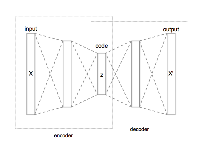
Figure 19.1: Schematic structure of an undercomplete autoencoder with three fully connected hidden layers .
To learn the neuron weights and, thus the codings, the autoencoder seeks to minimize some loss function, such as mean squared error (MSE), that penalizes \(X'\) for being dissimilar from \(X\):
\[\begin{equation} \tag{19.1} \text{minimize}\enspace L = f\left(X, X'\right) \end{equation}\]
19.2.1 Comparing PCA to an autoencoder
When the autoencoder uses only linear activation functions (reference Section 13.4.2.1) and the loss function is MSE, then it can be shown that the autoencoder reduces to PCA. When nonlinear activation functions are used, autoencoders provide nonlinear generalizations of PCA.
The following demonstrates our first implementation of a basic autoencoder. When using h2o you use the same h2o.deeplearning() function that you would use to train a neural network; however, you need to set autoencoder = TRUE. We use a single hidden layer with only two codings. This is reducing 784 features down to two dimensions; although not very realistic, it allows us to visualize the results and gain some intuition on the algorithm. In this example we use a hyperbolic tangent activation function which has a nonlinear sigmoidal shape. To extract the reduced dimension codings, we use h2o.deepfeatures() and specify the layer of codings to extract.
The MNIST data set is very sparse; in fact, over 80% of the elements in the MNIST data set are zeros. When you have sparse data such as this, using sparse = TRUE enables h2o to more efficiently handle the input data and speed up computation.
# Convert mnist features to an h2o input data set
features <- as.h2o(mnist$train$images)

# Train an autoencoder
ae1 <- h2o.deeplearning(
  x = seq_along(features),
  training_frame = features,
  autoencoder = TRUE,
  hidden = 2,
  activation = 'Tanh',
  sparse = TRUE
)

# Extract the deep features
ae1_codings <- h2o.deepfeatures(ae1, features, layer = 1)
ae1_codings
##     DF.L1.C1    DF.L1.C2
## 1 -0.1558956 -0.06456967
## 2  0.3778544 -0.61518649
## 3  0.2002303  0.31214266
## 4 -0.6955515  0.13225607
## 5  0.1912538  0.59865392
## 6  0.2310982  0.20322605
##
## [60000 rows x 2 columns]
The reduced codings we extract are sometimes referred to as deep features (DF) and they are similar in nature to the principal components for PCA and archetypes for GLRMs. In fact, we can project the MNIST response variable onto the reduced feature space and compare our autoencoder to PCA. Figure 19.2 illustrates how the nonlinearity of autoencoders can help to isolate the signals in the features better than PCA.
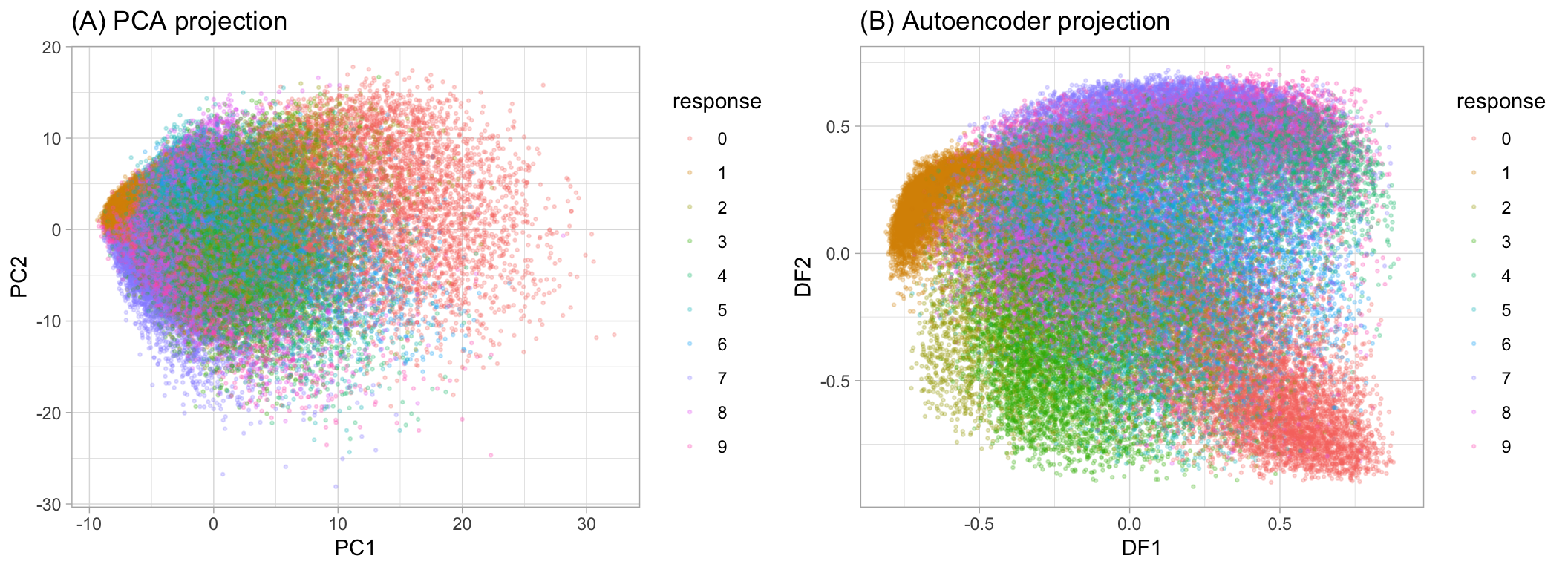
Figure 19.2: MNIST response variable projected onto a reduced feature space containin only two dimensions. PCA (left) forces a linear projection whereas an autoencoder with non-linear activation functions allows non-linear project.
19.2.2 Stacked autoencoders
Autoencoders are often trained with only a single hidden layer; however, this is not a requirement. Just as we illustrated with feedforward neural networks, autoencoders can have multiple hidden layers. We refer to autoencoders with more than one layer as stacked autoencoders (or deep autoencoders). Adding additional layers to autoencoders can have advantages. Adding additional depth can allow the codings to represent more complex, nonlinear relationships at a reduced computational cost. In fact, Hinton and Salakhutdinov (2006) show that deeper autoencoders often yield better data compression than shallower, or linear autoencoders. However, this is not always the case as we’ll see shortly.
One must be careful not to make the autoencoder too complex and powerful as you can run the risk of nearly reconstructing the inputs perfectly while not identifying the salient features that generalize well.
As you increase the depth of an autoencoder, the architecture typically follows a symmetrical pattern.47 For example, Figure 19.3 illustrates three different undercomplete autoencoder architectures exhibiting symmetric hidden layers.
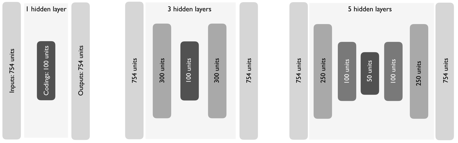
Figure 19.3: As you add hidden layers to autoencoders, it is common practice to have symmetric hidden layer sizes between the encoder and decoder layers.
So how does one find the right autencoder architecture? We can use the same grid search procedures we’ve discussed throughout the supervised learning section of the book. To illustrate, the following code examines five undercomplete autoencoder architectures. In this example we find that less depth provides the optimal MSE as a single hidden layer with 100 deep features has the lowest MSE of 0.007.
The following grid search took a little over 9 minutes.
# Hyperparameter search grid
hyper_grid <- list(hidden = list(
  c(50),
  c(100),
  c(300, 100, 300),
  c(100, 50, 100),
  c(250, 100, 50, 100, 250)
))

# Execute grid search
ae_grid <- h2o.grid(
  algorithm = 'deeplearning',
  x = seq_along(features),
  training_frame = features,
  grid_id = 'autoencoder_grid',
  autoencoder = TRUE,
  activation = 'Tanh',
  hyper_params = hyper_grid,
  sparse = TRUE,
  ignore_const_cols = FALSE,
  seed = 123
)

# Print grid details
h2o.getGrid('autoencoder_grid', sort_by = 'mse', decreasing = FALSE)
## H2O Grid Details
## ================
##
## Grid ID: autoencoder_grid
## Used hyper parameters:
##   -  hidden
## Number of models: 5
## Number of failed models: 0
##
## Hyper-Parameter Search Summary: ordered by increasing mse
##                     hidden                 model_ids                  mse
## 1                    [100] autoencoder_grid3_model_2  0.00674637890553651
## 2          [300, 100, 300] autoencoder_grid3_model_3  0.00830502966843272
## 3           [100, 50, 100] autoencoder_grid3_model_4 0.011215307972822733
## 4                     [50] autoencoder_grid3_model_1 0.012450109189122541
## 5 [250, 100, 50, 100, 250] autoencoder_grid3_model_5 0.014410280145600972
19.2.3 Visualizing the reconstruction
So how well does our autoencoder reconstruct the original inputs? The MSE provides us an overall error assessment but we can also directly compare the inputs and reconstructed outputs. Figure 19.4 illustrates this comparison by sampling a few test images, predicting the reconstructed pixel values based on our optimal autoencoder, and plotting the original versus reconstructed digits. The objective of the autoencoder is to capture the salient features of the images where any differences should be negligible; Figure 19.4 illustrates that our autencoder does a pretty good job of this.
# Get sampled test images
index <- sample(1:nrow(mnist$test$images), 4)
sampled_digits <- mnist$test$images[index, ]
colnames(sampled_digits) <- paste0("V", seq_len(ncol(sampled_digits)))

# Predict reconstructed pixel values
best_model_id <- ae_grid@model_ids[[1]]
best_model <- h2o.getModel(best_model_id)
reconstructed_digits <- predict(best_model, as.h2o(sampled_digits))
names(reconstructed_digits) <- paste0("V", seq_len(ncol(reconstructed_digits)))

combine <- rbind(sampled_digits, as.matrix(reconstructed_digits))

# Plot original versus reconstructed
par(mfrow = c(1, 3), mar=c(1, 1, 1, 1))
layout(matrix(seq_len(nrow(combine)), 4, 2, byrow = FALSE))
for(i in seq_len(nrow(combine))) {
  image(matrix(combine[i, ], 28, 28)[, 28:1], xaxt="n", yaxt="n")
}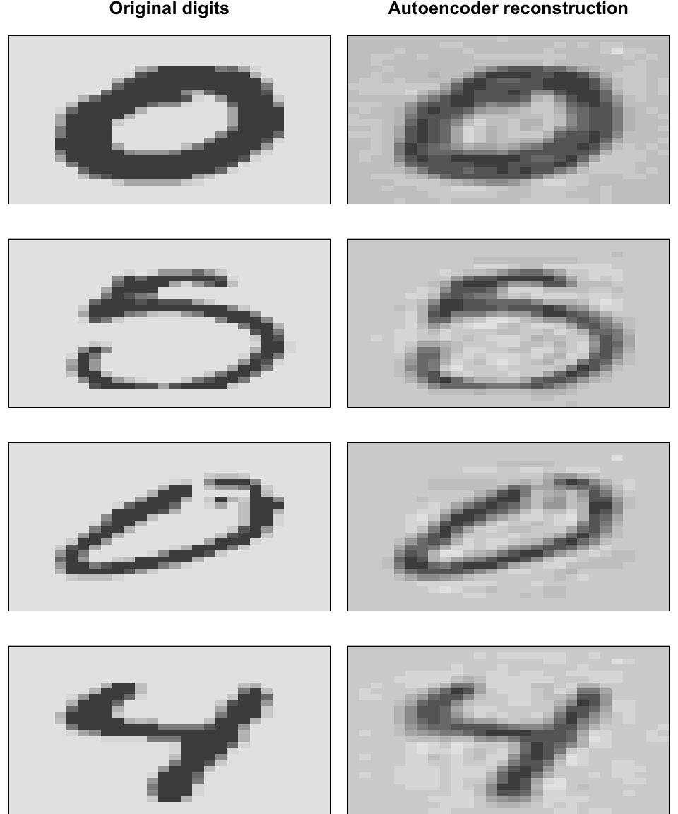
Figure 19.4: Original digits (left) and their reconstructions (right).
19.3 Sparse autoencoders
Sparse autoencoders are used to pull out the most influential feature representations. This is beneficial when trying to understand what are the most unique features of a data set. It’s useful when using autoencoders as inputs to downstream supervised models as it helps to highlight the unique signals across the features.
Recall that neurons in a network are considered active if the threshold exceeds certain capacity. Since a Tanh activation function is S-curved from -1 to 1, we consider a neuron active if the output value is closer to 1 and inactive if its output is closer to -1.48 Incorporating sparsity forces more neurons to be inactive. This requires the autoencoder to represent each input as a combination of a smaller number of activations. To incorporate sparsity, we must first understand the actual sparsity of the coding layer. This is simply the average activation of the coding layer as a function of the activation used (\(A\)) and the inputs supplied (\(X\)) as illustrated in Equation (19.2).
\[\begin{equation} \tag{19.2} \hat{\rho} = \frac{1}{m}\sum^m_{i=1}A(X) \end{equation}\]
For our current best_model with 100 codings, the sparsity level is approximately zero:
ae100_codings <- h2o.deepfeatures(best_model, features, layer = 1)
ae100_codings %>%
    as.data.frame() %>%
    tidyr::gather() %>%
    summarize(average_activation = mean(value))
##   average_activation
## 1        -0.00677801
This means, on average, the coding neurons are active half the time which is illustrated in Figure 19.5.
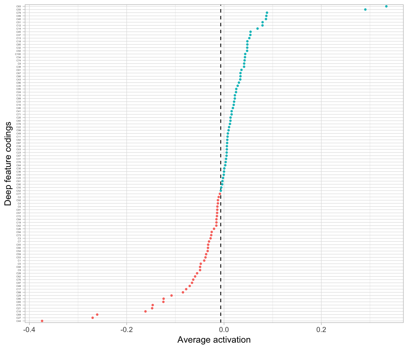
Figure 19.5: The average activation of the coding neurons in our default autoencoder using a Tanh activation function.
Sparse autoencoders attempt to enforce the constraint \(\widehat{\rho} = \rho\) where \(\rho\) is a sparsity parameter. This penalizes the neurons that are too active, forcing them to activate less. To achieve this we add an extra penalty term to our objective function in Equation (19.1). The most commonly used penalty is known as the Kullback-Leibler divergence (KL divergence), which will measure the divergence between the target probability \(\rho\) that a neuron in the coding layer will activate, and the actual probability as illustrated in Equation (19.3).
\[\begin{equation} \tag{19.3} \sum \rho \log \frac{\rho}{\hat\rho} + (1-\rho) \log \frac{1 - \rho}{1 - \hat \rho} \end{equation}\]
This penalty term is commonly written as Equation (19.4)
\[\begin{equation} \tag{19.4} \sum \sum \text{KL} (\rho || \hat{\rho}). \end{equation}\]
Similar to the ridge and LASSO penalties discussed in Section 6.2, we add this penalty to our objective function and incorporate a parameter (\(\beta\)) to control the weight of the penalty. Consequently, our revised loss function with sparsity induced is
\[\begin{equation} \tag{19.5} \text{minimize} \left(L = f(X, X') + \beta \sum \text{KL} (\rho || \hat{\rho}) \right). \end{equation}\]
Assume we want to induce sparsity with our current autoencoder that contains 100 codings. We need to specify two parameters: \(\rho\) and \(\beta\). In this example, we’ll just induce a little sparsity and specify \(\rho = -0.1\) by including average_activation = -0.1. And since \(\beta\) could take on multiple values we’ll do a grid search across different sparsity_beta values. Our results indicate that \(\beta = 0.01\) performs best in reconstructing the original inputs.
The weight that controls the relative importance of the sparsity loss (\(\beta\)) is a hyperparameter that needs to be tuned. If this weight is too high, the model will stick closely to the target sparsity but suboptimally reconstruct the inputs. If the weight is too low, the model will mostly ignore the sparsity objective. A grid search helps to find the right balance.
# Hyperparameter search grid
hyper_grid <- list(sparsity_beta = c(0.01, 0.05, 0.1, 0.2))

# Execute grid search
ae_sparsity_grid <- h2o.grid(
  algorithm = 'deeplearning',
  x = seq_along(features),
  training_frame = features,
  grid_id = 'sparsity_grid',
  autoencoder = TRUE,
  hidden = 100,
  activation = 'Tanh',
  hyper_params = hyper_grid,
  sparse = TRUE,
  average_activation = -0.1,
  ignore_const_cols = FALSE,
  seed = 123
)

# Print grid details
h2o.getGrid('sparsity_grid', sort_by = 'mse', decreasing = FALSE)
## H2O Grid Details
## ================
##
## Grid ID: sparsity_grid
## Used hyper parameters:
##   -  sparsity_beta
## Number of models: 4
## Number of failed models: 0
##
## Hyper-Parameter Search Summary: ordered by increasing mse
##   sparsity_beta             model_ids                  mse
## 1          0.01 sparsity_grid_model_1 0.012982916169006953
## 2           0.2 sparsity_grid_model_4  0.01321464889160263
## 3          0.05 sparsity_grid_model_2  0.01337749148043942
## 4           0.1 sparsity_grid_model_3 0.013516631653257992
If we look at the average activation across our neurons now we see that it shifted to the left compared to Figure 19.5; it is now -0.108 as illustrated in Figure 19.6.
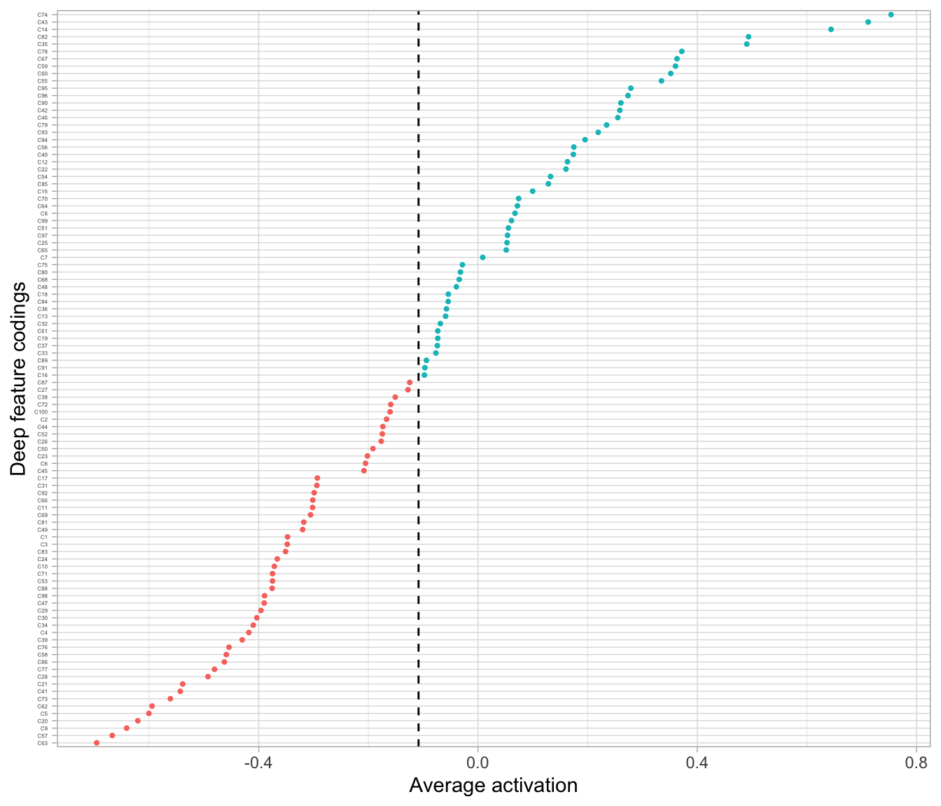
Figure 19.6: The average activation of the coding neurons in our sparse autoencoder is now -0.108.
The amount of sparsity you apply is dependent on multiple factors. When using autoencoders for descriptive dimension reduction, the level of sparsity is dependent on the level of insight you want to gain behind the most unique statistical features. If you’re trying to understand the most essential characteristics that explain the features or images then a lower sparsity value is preferred. For example, Figure 19.7 compares the four sampled digits from the MNIST test set with a non-sparse autoencoder with a single layer of 100 codings using Tanh activation functions and a sparse autoencoder that constrains \(\rho = -0.75\). Adding sparsity helps to highlight the features that are driving the uniqueness of these sampled digits. This is most pronounced with the number 5 where the sparse autoencoder reveals the primary focus is on the upper portion of the glyph.
If you are using autoencoders as a feature engineering step prior to downstream supervised modeling, then the level of sparsity can be considered a hyperparameter that can be optimized with a search grid.
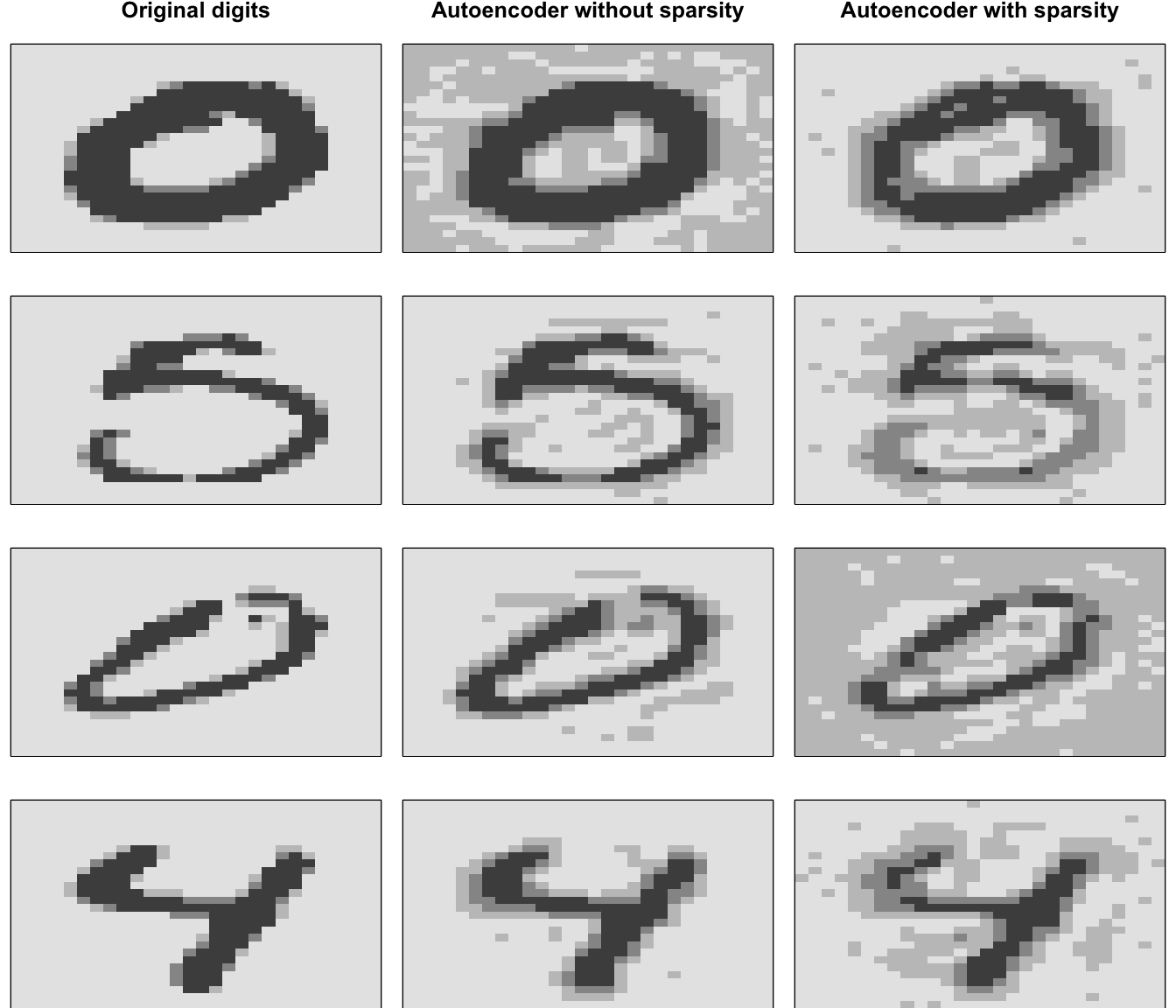
Figure 19.7: Original digits sampled from the MNIST test set (left), reconstruction of sampled digits with a non-sparse autoencoder (middle), and reconstruction with a sparse autoencoder (right).
In Section 19.2, we discussed how an undercomplete autoencoder is used to constrain the number of codings to be less than the number of inputs. This constraint prevents the autoencoder from learning the identify function, which would just create a perfect mapping of inputs to outputs and not learn anything about the features’ salient characteristics. However, there are ways to prevent an autoencoder with more hidden units than inputs (known as an overcomplete autoencoder) from learning the identity function. Adding sparsity is one such approach (Poultney et al. 2007; Lee, Ekanadham, and Ng 2008) and another is to add randomness in the transformation from input to reconstruction, which we discuss next.
19.4 Denoising autoencoders
The denoising autoencoder is a stochastic version of the autoencoder in which we train the autoencoder to reconstruct the input from a corrupted copy of the inputs. This forces the codings to learn more robust features of the inputs and prevents them from merely learning the identity function; even if the number of codings is greater than the number of inputs. We can think of a denoising autoencoder as having two objectives: (i) try to encode the inputs to preserve the essential signals, and (ii) try to undo the effects of a corruption process stochastically applied to the inputs of the autoencoder. The latter can only be done by capturing the statistical dependencies between the inputs. Combined, this denoising procedure allows us to implicitly learn useful properties of the inputs (Bengio et al. 2013).
The corruption process typically follows one of two approaches. We can randomly set some of the inputs (as many as half of them) to zero or one; most commonly it is setting random values to zero to imply missing values (Vincent et al. 2008). This can be done by manually imputing zeros or ones into the inputs or adding a dropout layer (reference Section 13.7.3) between the inputs and first hidden layer. Alternatively, for continuous-valued inputs, we can add pure Gaussian noise (Vincent 2011). Figure 19.8 illustrates the differences between these two corruption options for a sampled input where 30% of the inputs were corrupted.
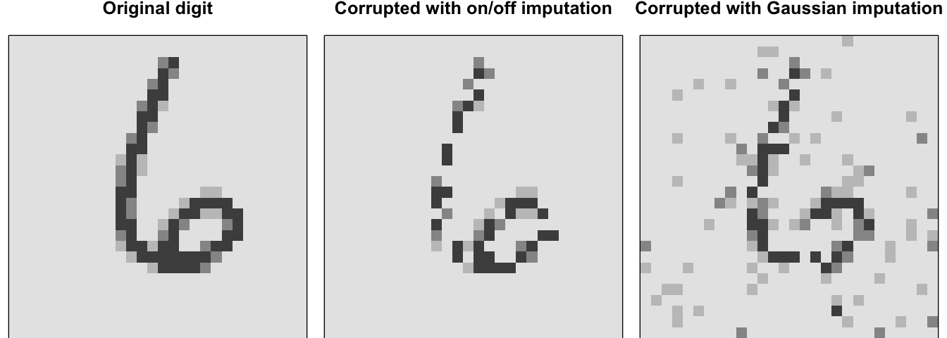
Figure 19.8: Original digit sampled from the MNIST test set (left), corrupted data with on/off imputation (middle), and corrupted data with Gaussian imputation (right).
Training a denoising autoencoder is nearly the same process as training a regular autoencoder. The only difference is we supply our corrupted inputs to training_frame and supply the non-corrupted inputs to validation_frame. The following code illustrates where we supply training_frame with inputs that have been corrupted with Gaussian noise (inputs_currupted_gaussian) and supply the original input data frame (features) to validation_frame. The remaining process stays, essentially, the same. We see that the validation MSE is 0.02 where in comparison our MSE of the same model without corrupted inputs was 0.006.
# Train a denoise autoencoder
denoise_ae <- h2o.deeplearning(
  x = seq_along(features),
  training_frame = inputs_currupted_gaussian,
  validation_frame = features,
  autoencoder = TRUE,
  hidden = 100,
  activation = 'Tanh',
  sparse = TRUE
)

# Print performance
h2o.performance(denoise_ae, valid = TRUE)
## H2OAutoEncoderMetrics: deeplearning
## ** Reported on validation data. **
##
## Validation Set Metrics:
## =====================
##
## MSE: (Extract with `h2o.mse`) 0.02048465
## RMSE: (Extract with `h2o.rmse`) 0.1431246
Figure 19.9 visualizes the effect of a denoising autoencoder. The left column shows a sample of the original digits, which are used as the validation data set. The middle column shows the Gaussian corrupted inputs used to train the model, and the right column shows the reconstructed digits after denoising. As expected, the denoising autoencoder does a pretty good job of mapping the corrupted data back to the original input.
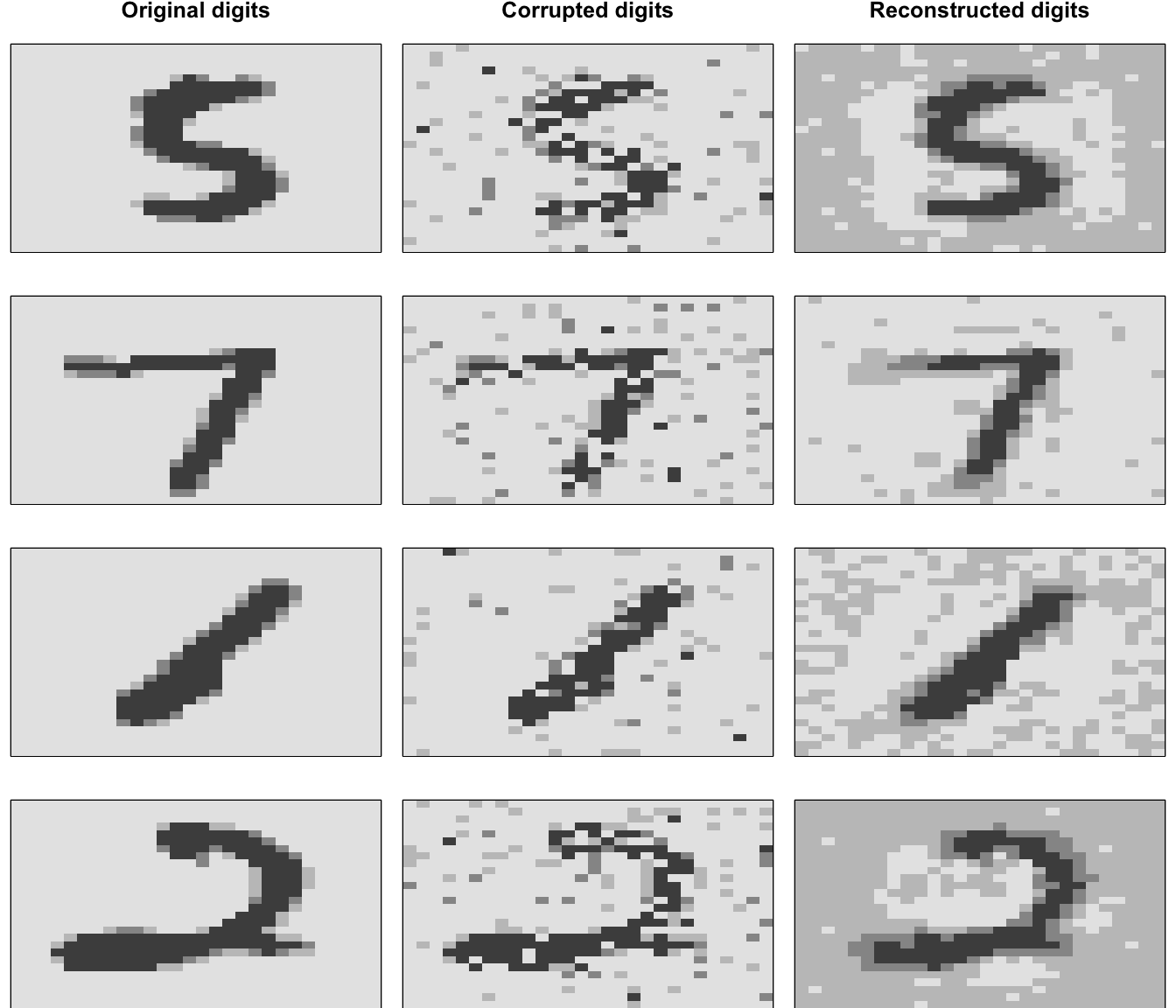
Figure 19.9: Original digits sampled from the MNIST test set (left), corrupted input digits (middle), and reconstructed outputs (right).
19.5 Anomaly detection
We can also use autoencoders for anomaly detection (Sakurada and Yairi 2014; Zhou and Paffenroth 2017). Since the loss function of an autoencoder measures the reconstruction error, we can extract this information to identify those observations that have larger error rates. These observations have feature attributes that differ significantly from the other features. We might consider such features as anomalous, or outliers.
To extract the reconstruction error with h2o, we use h2o.anomaly(). The following uses our undercomplete autoencoder with 100 codings from Section 19.2.2. We can see that the distribution of reconstruction errors range from near zero to over 0.03 with the average error being 0.006.
# Extract reconstruction errors
(reconstruction_errors <- h2o.anomaly(best_model, features))
##   Reconstruction.MSE
## 1        0.009879666
## 2        0.006485201
## 3        0.017470110
## 4        0.002339352
## 5        0.006077669
## 6        0.007171287
##
## [60000 rows x 1 column]

# Plot distribution
reconstruction_errors <- as.data.frame(reconstruction_errors)
ggplot(reconstruction_errors, aes(Reconstruction.MSE)) +
  geom_histogram()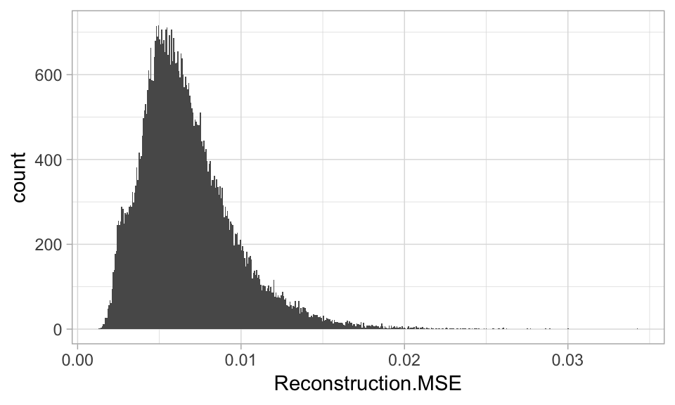
Figure 19.10: Distribution of reconstruction errors.
Figure 19.11 illustrates the actual and reconstructed digits for the observations with the five worst reconstruction errors. It is fairly intuitive why these observations have such large reconstruction errors as the corresponding input digits are poorly written.
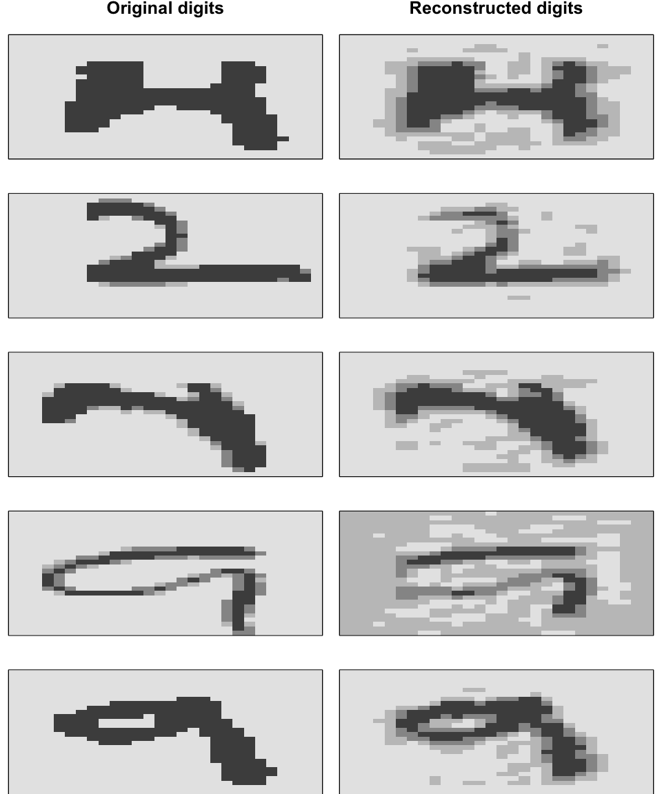
Figure 19.11: Original digits (left) and their reconstructions (right) for the observations with the five largest reconstruction errors.
In addition to identifying outliers, we can also use anomaly detection to identify unusual inputs such as fraudulent credit card transactions and manufacturing defects. Often, when performing anomaly detection, we retrain the autoencoder on a subset of the inputs that we’ve determined are a good representation of high quality inputs. For example, we may include all inputs that achieved a reconstruction error within the 75-th percentile and exclude the rest. We would then retrain an autoencoder, use that autoencoder on new input data, and if it exceeds a certain percentile declare the inputs as anomalous. However, deciding on the threshold that determines an input as anomalous is subjective and often relies on the business purpose.
19.6 Final thoughts
As we mentioned at the beginning of this chapter, autoencoders are receiving a lot of attention and many advancements have been made over the past decade. We discussed a few of the fundamental implementations of autoencoders; however, more exist. The following is an incomplete list of alternative autoencoders that are worthy of your attention.
- Variational autoencoders are a form of generative autoencoders, which means they can be used to create new instances that closely resemble the input data but are completely generated from the coding distributions (Doersch 2016).
- Contractive autoencoders constrain the derivative of the hidden layer(s) activations to be small with respect to the inputs. This has a similar effect as denoising autoencoders in the sense that small perturbations to the input are essentially considered noise, which makes our codings more robust (Rifai et al. 2011).
- Stacked convolutional autoencoders are designed to reconstruct visual features processed through convolutional layers (Masci et al. 2011). They do not require manual vectorization of the image so they work well if you need to do dimension reduction or feature extraction on realistic-sized high-dimensional images.
- Winner-take-all autoencoders leverage only the top X% activations for each neuron, while the rest are set to zero (Makhzani and Frey 2015). This leads to sparse codings. This approach has also been adapted to work with convolutional autoencoders (Makhzani and Frey 2014).
- Adversarial autoencoders train two networks - a generator network to reconstruct the inputs similar to a regular autoencoder and then a discriminator network to compute where the inputs lie on a probabilistic distribution. Similar to variational autoencoders, adversarial autoencoders are often used to generate new data and have also been used for semi-supervised and supervised tasks (Makhzani et al. 2015).
References
Bengio, Yoshua, Li Yao, Guillaume Alain, and Pascal Vincent. 2013. “Generalized Denoising Auto-Encoders as Generative Models.” In Advances in Neural Information Processing Systems, 899–907.
Bourlard, Hervé, and Yves Kamp. 1988. “Auto-Association by Multilayer Perceptrons and Singular Value Decomposition.” Biological Cybernetics 59 (4-5). Springer: 291–94.
Doersch, Carl. 2016. “Tutorial on Variational Autoencoders.” arXiv Preprint arXiv:1606.05908.
Hinton, Geoffrey E, and Ruslan R Salakhutdinov. 2006. “Reducing the Dimensionality of Data with Neural Networks.” Science 313 (5786). American Association for the Advancement of Science: 504–7.
Hinton, Geoffrey E, and Richard S Zemel. 1994. “Autoencoders, Minimum Description Length and Helmholtz Free Energy.” In Advances in Neural Information Processing Systems, 3–10.
LeCun, Yann. 1987. “Modeles Connexionnistes de L’apprentissage (Connectionist Learning Models).” Ph.D. thesis, Universite P. et M. Curie (Paris 6).
Lee, Honglak, Chaitanya Ekanadham, and Andrew Y Ng. 2008. “Sparse Deep Belief Net Model for Visual Area V2.” In Advances in Neural Information Processing Systems, 873–80.
Makhzani, Alireza, and Brendan Frey. 2014. “A Winner-Take-All Method for Training Sparse Convolutional Autoencoders.” In NIPS Deep Learning Workshop. Citeseer.
Makhzani, Alireza, and Brendan J Frey. 2015. “Winner-Take-All Autoencoders.” In Advances in Neural Information Processing Systems, 2791–9.
Makhzani, Alireza, Jonathon Shlens, Navdeep Jaitly, Ian Goodfellow, and Brendan Frey. 2015. “Adversarial Autoencoders.” arXiv Preprint arXiv:1511.05644.
Masci, Jonathan, Ueli Meier, Dan Cireşan, and Jürgen Schmidhuber. 2011. “Stacked Convolutional Auto-Encoders for Hierarchical Feature Extraction.” In International Conference on Artificial Neural Networks, 52–59. Springer.
Poultney, Christopher, Sumit Chopra, Yann L Cun, and others. 2007. “Efficient Learning of Sparse Representations with an Energy-Based Model.” In Advances in Neural Information Processing Systems, 1137–44.
Rifai, Salah, Pascal Vincent, Xavier Muller, Xavier Glorot, and Yoshua Bengio. 2011. “Contractive Auto-Encoders: Explicit Invariance During Feature Extraction.” In Proceedings of the 28th International Conference on International Conference on Machine Learning, 833–40. Omnipress.
Sakurada, Mayu, and Takehisa Yairi. 2014. “Anomaly Detection Using Autoencoders with Nonlinear Dimensionality Reduction.” In Proceedings of the Mlsda 2014 2nd Workshop on Machine Learning for Sensory Data Analysis, 4. ACM.
Vincent, Pascal. 2011. “A Connection Between Score Matching and Denoising Autoencoders.” Neural Computation 23 (7). MIT Press: 1661–74.
Vincent, Pascal, Hugo Larochelle, Yoshua Bengio, and Pierre-Antoine Manzagol. 2008. “Extracting and Composing Robust Features with Denoising Autoencoders.” In Proceedings of the 25th Iternational Conference on Machine Learning, 1096–1103. ACM.
Zhou, Chong, and Randy C Paffenroth. 2017. “Anomaly Detection with Robust Deep Autoencoders.” In Proceedings of the 23rd Acm Sigkdd International Conference on Knowledge Discovery and Data Mining, 665–74. ACM.