Chapter 7 Multivariate Adaptive Regression Splines

The previous chapters discussed algorithms that are intrinsically linear. Many of these models can be adapted to nonlinear patterns in the data by manually adding nonlinear model terms (e.g., squared terms, interaction effects, and other transformations of the original features); however, to do so you the analyst must know the specific nature of the nonlinearities and interactions a priori. Alternatively, there are numerous algorithms that are inherently nonlinear. When using these models, the exact form of the nonlinearity does not need to be known explicitly or specified prior to model training. Rather, these algorithms will search for, and discover, nonlinearities and interactions in the data that help maximize predictive accuracy.

This chapter discusses multivariate adaptive regression splines (MARS) (Friedman 1991), an algorithm that automatically creates a piecewise linear model which provides an intuitive stepping block into nonlinearity after grasping the concept of multiple linear regression. Future chapters will focus on other nonlinear algorithms.

7.1 Prerequisites

For this chapter we will use the following packages:

# Helper packages
library(dplyr)     # for data wrangling
library(ggplot2)   # for awesome plotting

# Modeling packages
library(earth)     # for fitting MARS models
library(caret)     # for automating the tuning process

# Model interpretability packages
library(vip)       # for variable importance
library(pdp)       # for variable relationships

To illustrate various concepts we’ll continue with the ames_train and ames_test data sets created in Section 2.7.

7.2 The basic idea

In the previous chapters, we focused on linear models (where the analyst has to explicitly specify any nonlinear relationships and interaction effects). We illustrated some of the advantages of linear models such as their ease and speed of computation and also the intuitive nature of interpreting their coefficients. However, linear models make a strong assumption about linearity, and this assumption is often a poor one, which can affect predictive accuracy.

We can extend linear models to capture any non-linear relationship. Typically, this is done by explicitly including polynomial terms (e.g., $x_i^2$) or step functions. Polynomial regression is a form of regression in which the relationship between $X$ and $Y$ is modeled as a $d$th degree polynomial in $X$. For example, Equation (7.1) represents a polynomial regression function where $Y$ is modeled as a $d$-th degree polynomial in $X$. Generally speaking, it is unusual to use $d$ greater than 3 or 4 as the larger $d$ becomes, the easier the function fit becomes overly flexible and oddly shaped…especially near the boundaries of the range of $X$ values. Increasing $d$ also tends to increase the presence of multicollinearity.

\[\begin{equation} \tag{7.1} y_i = \beta_0 + \beta_1 x_i + \beta_2 x^2_i + \beta_3 x^3_i \dots + \beta_d x^d_i + \epsilon_i, \end{equation}\]

An alternative to polynomials is to use step functions. Whereas polynomial functions impose a global non-linear relationship, step functions break the range of $X$ into bins, and fit a simple constant (e.g., the mean response) in each. This amounts to converting a continuous feature into an ordered categorical variable such that our linear regression function is converted to Equation (7.2)

\[\begin{equation} \tag{7.2} y_i = \beta_0 + \beta_1 C_1(x_i) + \beta_2 C_2(x_i) + \beta_3 C_3(x_i) \dots + \beta_d C_d(x_i) + \epsilon_i, \end{equation}\]

where $C_1(x_i)$ represents $x_i$ values ranging from $c_1 \leq x_i < c_2$, $C_2\left(x_i\right)$ represents $x_i$ values ranging from $c_2 \leq x_i < c_3$, $\dots$, $C_d\left(x_i\right)$ represents $x_i$ values ranging from $c_{d-1} \leq x_i < c_d$. Figure 7.1 contrasts linear, polynomial, and step function fits for non-linear, non-monotonic simulated data.

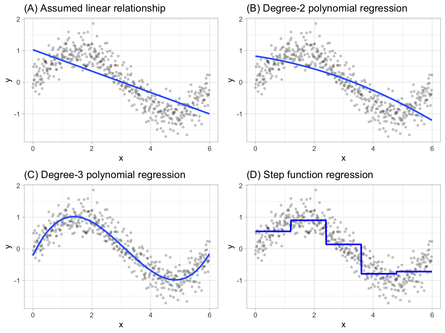
Blue line represents predicted (`y`) values as a function of `x` for alternative approaches to modeling explicit nonlinear regression patterns. (A) Traditional linear regression approach does not capture any nonlinearity unless the predictor or response is transformed (i.e. log transformation). (B) Degree-2 polynomial, (C) Degree-3 polynomial, (D) Step function cutting `x` into six categorical levels.

Figure 7.1: Blue line represents predicted (y) values as a function of x for alternative approaches to modeling explicit nonlinear regression patterns. (A) Traditional linear regression approach does not capture any nonlinearity unless the predictor or response is transformed (i.e. log transformation). (B) Degree-2 polynomial, (C) Degree-3 polynomial, (D) Step function cutting x into six categorical levels.

Although useful, the typical implementation of polynomial regression and step functions require the user to explicitly identify and incorporate which variables should have what specific degree of interaction or at what points of a variable $X$ should cut points be made for the step functions. Considering many data sets today can easily contain 50, 100, or more features, this would require an enormous and unnecessary time commitment from an analyst to determine these explicit non-linear settings.

7.2.1 Multivariate adaptive regression splines

Multivariate adaptive regression splines (MARS) provide a convenient approach to capture the nonlinear relationships in the data by assessing cutpoints (knots) similar to step functions. The procedure assesses each data point for each predictor as a knot and creates a linear regression model with the candidate feature(s). For example, consider our non-linear, non-monotonic data above where $Y = f\left(X\right)$. The MARS procedure will first look for the single point across the range of X values where two different linear relationships between Y and X achieve the smallest error (e.g., smallest SSE). What results is known as a hinge function $h\left(x-a\right)$, where $a$ is the cutpoint value. For a single knot (Figure 7.2 (A)), our hinge function is $h\left(\text{x}-1.183606\right)$ such that our two linear models for Y are

\[\begin{equation} \tag{7.3} \text{y} = \begin{cases} \beta_0 + \beta_1(1.183606 - \text{x}) & \text{x} < 1.183606, \\ \beta_0 + \beta_1(\text{x} - 1.183606) & \text{x} > 1.183606 \end{cases} \end{equation}\]

Once the first knot has been found, the search continues for a second knot which is found at $x = 4.898114$ (Figure 7.2 (B)). This results in three linear models for y:

\[\begin{equation} \tag{7.4} \text{y} = \begin{cases} \beta_0 + \beta_1(1.183606 - \text{x}) & \text{x} < 1.183606, \\ \beta_0 + \beta_1(\text{x} - 1.183606) & \text{x} > 1.183606 \quad \& \quad \text{x} < 4.898114, \\ \beta_0 + \beta_1(4.898114 - \text{x}) & \text{x} > 4.898114 \end{cases} \end{equation}\]

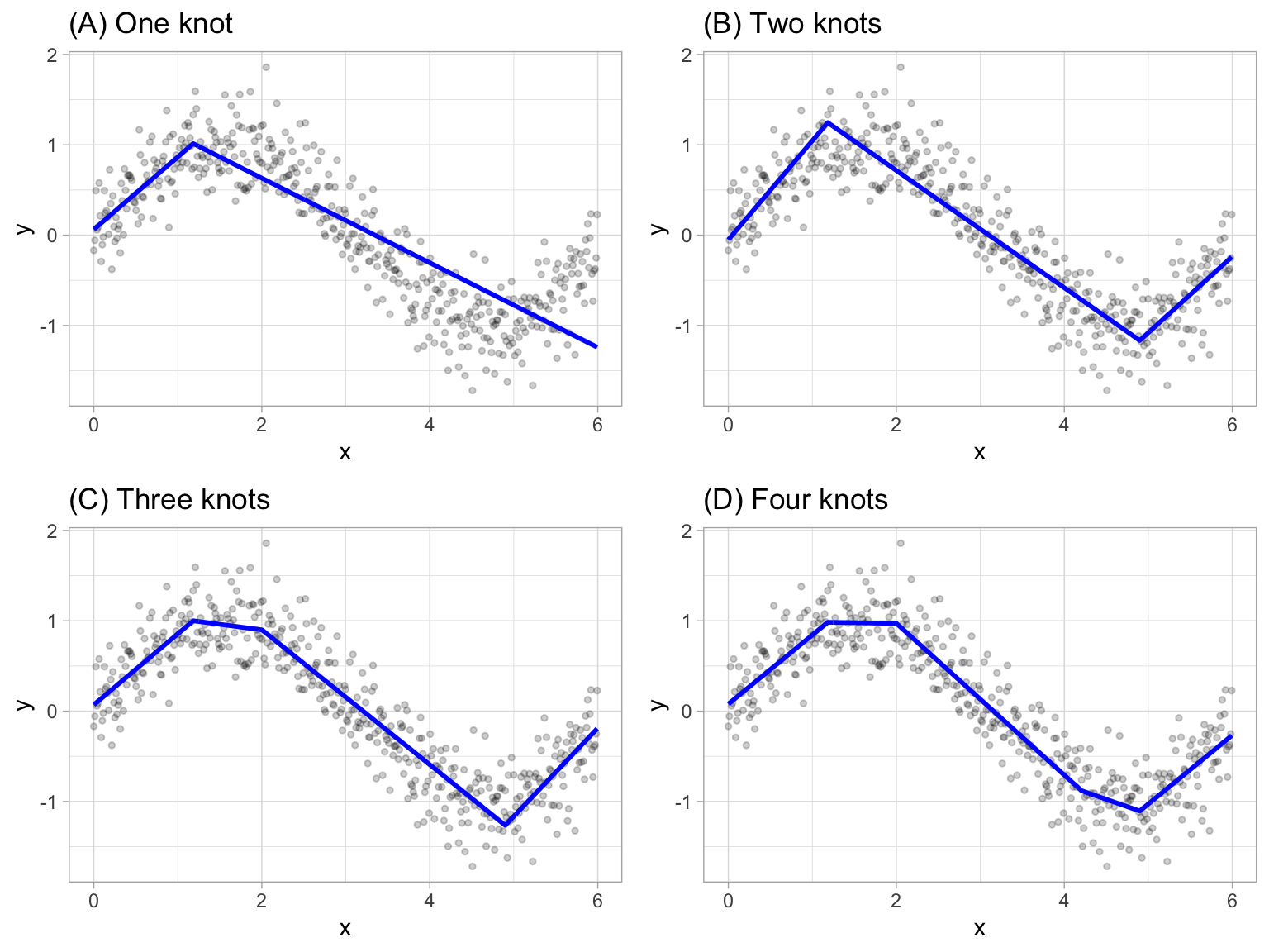
Figure 7.2: Examples of fitted regression splines of one (A), two (B), three (C), and four (D) knots.

This procedure continues until many knots are found, producing a (potentially) highly non-linear prediction equation. Although including many knots may allow us to fit a really good relationship with our training data, it may not generalize very well to new, unseen data. Consequently, once the full set of knots has been identified, we can sequentially remove knots that do not contribute significantly to predictive accuracy. This process is known as “pruning” and we can use cross-validation, as we have with the previous models, to find the optimal number of knots.

7.3 Fitting a basic MARS model

We can fit a direct engine MARS model with the earth package (Trevor Hastie and Thomas Lumley’s leaps wrapper. 2019). By default, earth::earth() will assess all potential knots across all supplied features and then will prune to the optimal number of knots based on an expected change in $R^2$ (for the training data) of less than 0.001. This calculation is performed by the Generalized cross-validation (GCV) procedure, which is a computational shortcut for linear models that produces an approximate leave-one-out cross-validation error metric (Golub, Heath, and Wahba 1979).

The term “MARS” is trademarked and licensed exclusively to Salford Systems: https://www.salford-systems.com. We can use MARS as an abbreviation; however, it cannot be used for competing software solutions. This is why the R package uses the name earth. Although, according to the package documentation, a backronym for “earth” is “Enhanced Adaptive Regression Through Hinges”.

The following applies a basic MARS model to our ames example. The results show us the final models GCV statistic, generalized $R^2$ (GRSq), and more.

# Fit a basic MARS model
mars1 <- earth(
  Sale_Price ~ .,  
  data = ames_train   
)

# Print model summary
print(mars1)
## Selected 36 of 39 terms, and 27 of 307 predictors
## Termination condition: RSq changed by less than 0.001 at 39 terms
## Importance: Gr_Liv_Area, Year_Built, Total_Bsmt_SF, ...
## Number of terms at each degree of interaction: 1 35 (additive model)
## GCV 557038757    RSS 1.065869e+12    GRSq 0.9136059    RSq 0.9193997

It also shows us that 36 of 39 terms were used from 27 of the 307 original predictors. But what does this mean? If we were to look at all the coefficients, we would see that there are 36 terms in our model (including the intercept). These terms include hinge functions produced from the original 307 predictors (307 predictors because the model automatically dummy encodes categorical features). Looking at the first 10 terms in our model, we see that Gr_Liv_Area is included with a knot at 2787 (the coefficient for $h\left(2787-\text{Gr_Liv_Area}\right)$ is -50.84), Year_Built is included with a knot at 2004, etc.

You can check out all the coefficients with summary(mars1) or coef(mars1).

summary(mars1) %>% .$coefficients %>% head(10)
##                              Sale_Price
## (Intercept)                223113.83301
## h(2787-Gr_Liv_Area)           -50.84125
## h(Year_Built-2004)           3405.59787
## h(2004-Year_Built)           -382.79774
## h(Total_Bsmt_SF-1302)          56.13784
## h(1302-Total_Bsmt_SF)         -29.72017
## h(Bsmt_Unf_SF-534)            -24.36493
## h(534-Bsmt_Unf_SF)             16.61145
## Overall_QualExcellent       80543.25421
## Overall_QualVery_Excellent 118297.79515

The plot method for MARS model objects provides useful performance and residual plots. Figure 7.3 illustrates the model selection plot that graphs the GCV $R^2$ (left-hand $y$-axis and solid black line) based on the number of terms retained in the model ($x$-axis) which are constructed from a certain number of original predictors (right-hand $y$-axis). The vertical dashed lined at 36 tells us the optimal number of terms retained where marginal increases in GCV $R^2$ are less than 0.001.

plot(mars1, which = 1)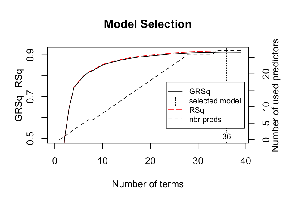

Model summary capturing GCV $R^2$ (left-hand y-axis and solid black line) based on the number of terms retained (x-axis) which is based on the number of predictors used to make those terms (right-hand side y-axis). For this model, 35 non-intercept terms were retained which are based on 27 predictors. Any additional terms retained in the model, over and above these 35, result in less than 0.001 improvement in the GCV $R^2$.

Figure 7.3: Model summary capturing GCV $R^2$ (left-hand y-axis and solid black line) based on the number of terms retained (x-axis) which is based on the number of predictors used to make those terms (right-hand side y-axis). For this model, 35 non-intercept terms were retained which are based on 27 predictors. Any additional terms retained in the model, over and above these 35, result in less than 0.001 improvement in the GCV $R^2$.

In addition to pruning the number of knots, earth::earth() allows us to also assess potential interactions between different hinge functions. The following illustrates this by including a degree = 2 argument. You can see that now our model includes interaction terms between a maximum of two hinge functions (e.g., h(2004-Year_Built)*h(Total_Bsmt_SF-1330) represents an interaction effect for those houses built after 2004 and has more than 1,330 square feet of basement space).

# Fit a basic MARS model
mars2 <- earth(
  Sale_Price ~ .,  
  data = ames_train,
  degree = 2
)

# check out the first 10 coefficient terms
summary(mars2) %>% .$coefficients %>% head(10)
##                                             Sale_Price
## (Intercept)                               2.331420e+05
## h(Gr_Liv_Area-2787)                       1.084015e+02
## h(2787-Gr_Liv_Area)                      -6.178182e+01
## h(Year_Built-2004)                        8.088153e+03
## h(2004-Year_Built)                       -9.529436e+02
## h(Total_Bsmt_SF-1302)                     1.131967e+02
## h(1302-Total_Bsmt_SF)                    -4.083722e+01
## h(2004-Year_Built)*h(Total_Bsmt_SF-1330) -1.553894e+00
## h(2004-Year_Built)*h(1330-Total_Bsmt_SF)  1.983699e-01
## Condition_1PosN*h(Gr_Liv_Area-2787)      -4.020535e+02

7.4 Tuning

There are two important tuning parameters associated with our MARS model: the maximum degree of interactions and the number of terms retained in the final model. We need to perform a grid search to identify the optimal combination of these hyperparameters that minimize prediction error (the above pruning process was based only on an approximation of CV model performance on the training data rather than an exact k-fold CV process). As in previous chapters, we’ll perform a CV grid search to identify the optimal hyperparameter mix. Below, we set up a grid that assesses 30 different combinations of interaction complexity (degree) and the number of terms to retain in the final model (nprune).

Rarely is there any benefit in assessing greater than 3-rd degree interactions and we suggest starting out with 10 evenly spaced values for nprune and then you can always zoom in to a region once you find an approximate optimal solution.

# create a tuning grid
hyper_grid <- expand.grid(
  degree = 1:3, 
  nprune = seq(2, 100, length.out = 10) %>% floor()
)

head(hyper_grid)
##   degree nprune
## 1      1      2
## 2      2      2
## 3      3      2
## 4      1     12
## 5      2     12
## 6      3     12

As in the previous chapters, we can use caret to perform a grid search using 10-fold CV. The model that provides the optimal combination includes second degree interaction effects and retains 56 terms. The cross-validated RMSE for these models is displayed in Figure 7.4; the optimal model’s cross-validated RMSE was $26,817.

This grid search took roughly five minutes to complete.

# Cross-validated model
set.seed(123)  # for reproducibility
cv_mars <- train(
  x = subset(ames_train, select = -Sale_Price),
  y = ames_train$Sale_Price,
  method = "earth",
  metric = "RMSE",
  trControl = trainControl(method = "cv", number = 10),
  tuneGrid = hyper_grid
)

# View results
cv_mars$bestTune
##    nprune degree
## 16     56      2

cv_mars$results %>%
  filter(nprune == cv_mars$bestTune$nprune, degree == cv_mars$bestTune$degree)
##   degree nprune    RMSE  Rsquared      MAE   RMSESD RsquaredSD    MAESD
## 1      2     56 26817.1 0.8838914 16439.15 11683.73 0.09785945 1678.672

ggplot(cv_mars)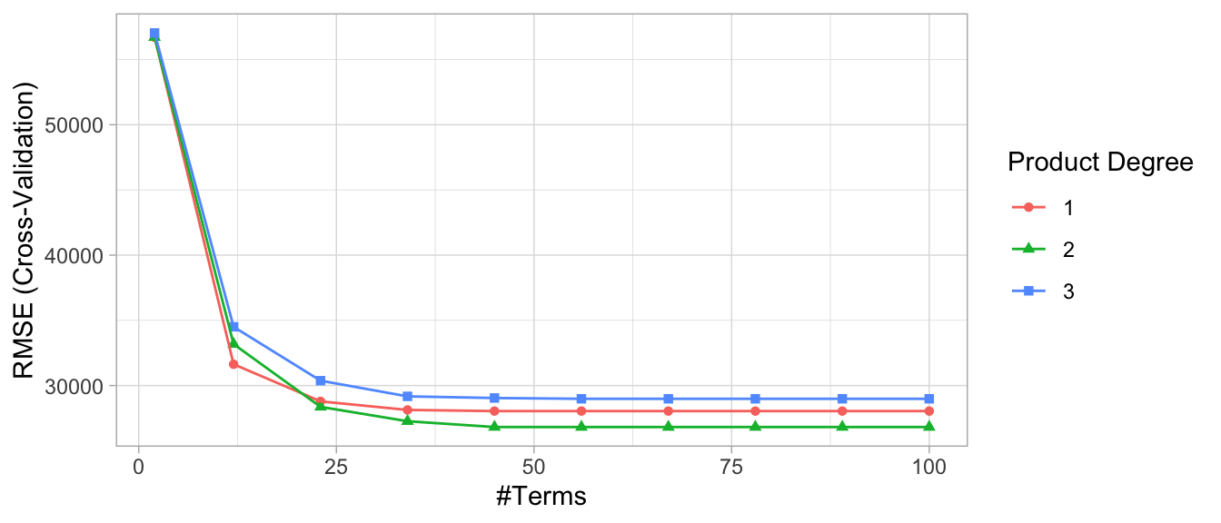

$Cross-validated RMSE for the 30 different hyperparameter combinations in our grid search. The optimal model retains 56 terms and includes up to 2$^{nd}$ degree interactions.$

Figure 7.4: Cross-validated RMSE for the 30 different hyperparameter combinations in our grid search. The optimal model retains 56 terms and includes up to 2$^{nd}$ degree interactions.

The above grid search helps to focus where we can further refine our model tuning. As a next step, we could perform a grid search that focuses in on a refined grid space for nprune (e.g., comparing 45–65 terms retained). However, for brevity we’ll leave this as an exercise for the reader.

So how does this compare to our previously built models for the Ames housing data? The following table compares the cross-validated RMSE for our tuned MARS model to an ordinary multiple regression model along with tuned principal component regression (PCR), partial least squares (PLS), and regularized regression (elastic net) models.

Notice that our elastic net model is higher than in the last chapter. This table compares these 5 modeling approaches without performing any logarithmic transformation on the target variable. However, our MARS model still outperforms the results from the best elastic net in the last chapter (RMSE = 19,905).

Table 7.1: Cross-validated RMSE results for tuned MARS and regression models.
	Min.	1st Qu.	Median	Mean	3rd Qu.	Max.
LM	16533.37	22621.51	24773.10	25957.46	28351.02	39572.36
PCR	28279.98	30963.21	31425.07	33871.79	36925.82	42676.08
PLS	16645.33	21832.43	24611.00	25296.77	25879.52	39231.40
ENET	15610.37	21035.04	23609.76	24647.70	25653.41	39184.22
MARS	19888.56	22240.22	23370.48	26817.10	24320.10	59443.17

Although the MARS model did not have a lower MSE than the elastic net and PLS models, you can see that the the median RMSE of all the cross validation iterations was lower. However, there is one fold (Fold08) that had an extremely large RMSE that is skewing the mean RMSE for the MARS model. This would be worth exploring as there are likely some unique observations that are skewing the results.

cv_mars$resample
##        RMSE  Rsquared      MAE Resample
## 1  22468.90 0.9205286 15471.14   Fold03
## 2  19888.56 0.9316275 14944.30   Fold04
## 3  59443.17 0.6143857 20867.67   Fold08
## 4  22163.99 0.9395510 16327.75   Fold07
## 5  24249.53 0.9278253 16551.83   Fold01
## 6  20711.49 0.9188620 15659.14   Fold05
## 7  23439.68 0.9241964 15463.52   Fold09
## 8  24343.62 0.9118472 16556.19   Fold02
## 9  28160.73 0.8513779 16955.07   Fold06
## 10 23301.28 0.8987123 15594.89   Fold10

7.5 Feature interpretation

MARS models via earth::earth() include a backwards elimination feature selection routine that looks at reductions in the GCV estimate of error as each predictor is added to the model. This total reduction is used as the variable importance measure (value = "gcv"). Since MARS will automatically include and exclude terms during the pruning process, it essentially performs automated feature selection. If a predictor was never used in any of the MARS basis functions in the final model (after pruning), it has an importance value of zero. This is illustrated in Figure 7.5 where 27 features have $>0$ importance values while the rest of the features have an importance value of zero since they were not included in the final model. Alternatively, you can also monitor the change in the residual sums of squares (RSS) as terms are added (value = "rss"); however, you will see very little difference between these methods.

# variable importance plots
p1 <- vip(cv_mars, num_features = 40, geom = "point", value = "gcv") + ggtitle("GCV")
p2 <- vip(cv_mars, num_features = 40, geom = "point", value = "rss") + ggtitle("RSS")

gridExtra::grid.arrange(p1, p2, ncol = 2)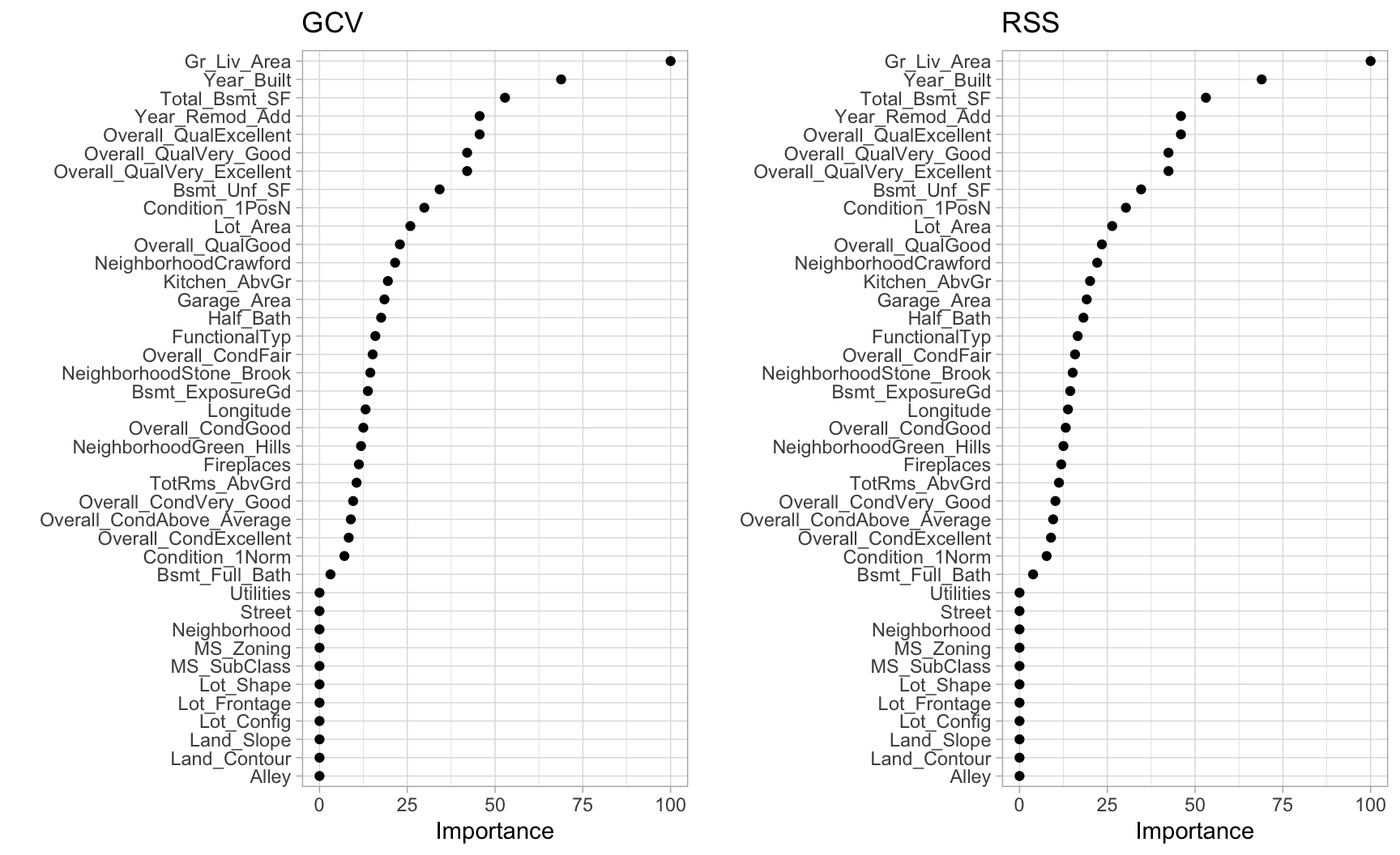

Variable importance based on impact to GCV (left) and RSS (right) values as predictors are added to the model. Both variable importance measures will usually give you very similar results.

Figure 7.5: Variable importance based on impact to GCV (left) and RSS (right) values as predictors are added to the model. Both variable importance measures will usually give you very similar results.

Its important to realize that variable importance will only measure the impact of the prediction error as features are included; however, it does not measure the impact for particular hinge functions created for a given feature. For example, in Figure 7.5 we see that Gr_Liv_Area and Year_Built are the two most influential variables; however, variable importance does not tell us how our model is treating the non-linear patterns for each feature. Also, if we look at the interaction terms our model retained, we see interactions between different hinge functions.

# extract coefficients, convert to tidy data frame, and
# filter for interaction terms
cv_mars$finalModel %>%
  coef() %>%  
  broom::tidy() %>%  
  filter(stringr::str_detect(names, "\\*")) 
## # A tibble: 20 x 2
##    names                                                       x
##    <chr>                                                   <dbl>
##  1 h(2004-Year_Built) * h(Total_Bsmt_SF-1330)           -1.55   
##  2 h(2004-Year_Built) * h(1330-Total_Bsmt_SF)            0.198  
##  3 Condition_1PosN * h(Gr_Liv_Area-2787)              -402.     
##  4 h(17871-Lot_Area) * h(Total_Bsmt_SF-1302)            -0.00703
##  5 h(Year_Built-2004) * h(2787-Gr_Liv_Area)             -4.54   
##  6 h(2004-Year_Built) * h(2787-Gr_Liv_Area)              0.135  
##  7 h(Year_Remod_Add-1973) * h(900-Garage_Area)          -1.61   
##  8 Overall_QualExcellent * h(Year_Remod_Add-1973)     2038.     
##  9 h(Total_Bsmt_SF-1302) * h(TotRms_AbvGrd-7)           12.2    
## 10 h(Total_Bsmt_SF-1302) * h(7-TotRms_AbvGrd)           30.6    
## 11 h(Total_Bsmt_SF-1302) * h(1-Half_Bath)              -35.6    
## 12 h(Lot_Area-6130) * Overall_CondFair                  -3.04   
## 13 NeighborhoodStone_Brook * h(Year_Remod_Add-1973)   1153.     
## 14 Overall_QualVery_Good * h(Bsmt_Full_Bath-1)       48011.     
## 15 Overall_QualVery_Good * h(1-Bsmt_Full_Bath)      -12239.     
## 16 Overall_CondGood * h(2004-Year_Built)               297.     
## 17 h(Year_Remod_Add-1973) * h(Longitude- -93.6571)   -9005.     
## 18 h(Year_Remod_Add-1973) * h(-93.6571-Longitude)   -14103.     
## 19 Overall_CondAbove_Average * h(2787-Gr_Liv_Area)       5.80   
## 20 Condition_1Norm * h(2004-Year_Built)                148.

To better understand the relationship between these features and Sale_Price, we can create partial dependence plots (PDPs) for each feature individually and also together. The individual PDPs illustrate that our model found that one knot in each feature provides the best fit. For example, as homes exceed 2,787 square feet, each additional square foot demands a higher marginal increase in sale price than homes with less than 2,787 square feet. Similarly, for homes built in 2004 or later, there is a greater marginal effect on sales price based on the age of the home than for homes built prior to 2004. The interaction plot (far right figure) illustrates the stronger effect these two features have when combined.

# Construct partial dependence plots
p1 <- partial(cv_mars, pred.var = "Gr_Liv_Area", grid.resolution = 10) %>% 
  autoplot()
p2 <- partial(cv_mars, pred.var = "Year_Built", grid.resolution = 10) %>% 
  autoplot()
p3 <- partial(cv_mars, pred.var = c("Gr_Liv_Area", "Year_Built"), 
              grid.resolution = 10) %>% 
  plotPartial(levelplot = FALSE, zlab = "yhat", drape = TRUE, colorkey = TRUE, 
              screen = list(z = -20, x = -60))

# Display plots side by side
gridExtra::grid.arrange(p1, p2, p3, ncol = 3)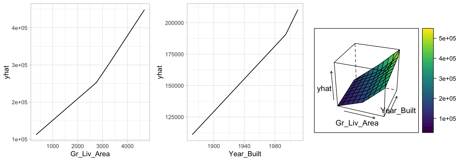

Partial dependence plots to understand the relationship between `Sale_Price` and the `Gr_Liv_Area` and `Year_Built` features. The PDPs tell us that as `Gr_Liv_Area` increases and for newer homes, `Sale_Price` increases dramatically.

Figure 7.6: Partial dependence plots to understand the relationship between Sale_Price and the Gr_Liv_Area and Year_Built features. The PDPs tell us that as Gr_Liv_Area increases and for newer homes, Sale_Price increases dramatically.

7.6 Attrition data

The MARS method and algorithm can be extended to handle classification problems and GLMs in general.²⁴ We saw significant improvement to our predictive accuracy on the Ames data with a MARS model, but how about the employee attrition example? In Chapter 5 we saw a slight improvement in our cross-validated accuracy rate using regularized regression. Here, we tune a MARS model using the same search grid as we did above. We see our best models include no interaction effects and the optimal model retained 12 terms.

# get attrition data
df <- rsample::attrition %>% mutate_if(is.ordered, factor, ordered = FALSE)

# Create training (70%) and test (30%) sets for the rsample::attrition data.
# Use set.seed for reproducibility
set.seed(123)
churn_split <- rsample::initial_split(df, prop = .7, strata = "Attrition")
churn_train <- rsample::training(churn_split)
churn_test  <- rsample::testing(churn_split)


# for reproducibiity
set.seed(123)

# cross validated model
tuned_mars <- train(
  x = subset(churn_train, select = -Attrition),
  y = churn_train$Attrition,
  method = "earth",
  trControl = trainControl(method = "cv", number = 10),
  tuneGrid = hyper_grid
)

# best model
tuned_mars$bestTune
##   nprune degree
## 2     12      1

# plot results
ggplot(tuned_mars)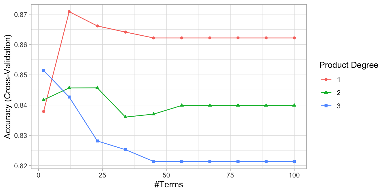

Cross-validated accuracy rate for the 30 different hyperparameter combinations in our grid search. The optimal model retains 12 terms and includes no interaction effects.

Figure 7.7: Cross-validated accuracy rate for the 30 different hyperparameter combinations in our grid search. The optimal model retains 12 terms and includes no interaction effects.

However, comparing our MARS model to the previous linear models (logistic regression and regularized regression), we do not see any improvement in our overall accuracy rate.

Table 7.2: Cross-validated accuracy results for tuned MARS and regression models.
	Min.	1st Qu.	Median	Mean	3rd Qu.	Max.
Logistic_model	0.8365385	0.8495146	0.8792476	0.8757893	0.8907767	0.9313725
Elastic_net	0.8446602	0.8759280	0.8834951	0.8835759	0.8915469	0.9411765
MARS_model	0.8155340	0.8578463	0.8780697	0.8708500	0.8907767	0.9029126

7.7 Final thoughts

There are several advantages to MARS. First, MARS naturally handles mixed types of predictors (quantitative and qualitative). MARS considers all possible binary partitions of the categories for a qualitative predictor into two groups.²⁵ Each group then generates a pair of piecewise indicator functions for the two categories. MARS also requires minimal feature engineering (e.g., feature scaling) and performs automated feature selection. For example, since MARS scans each predictor to identify a split that improves predictive accuracy, non-informative features will not be chosen. Furthermore, highly correlated predictors do not impede predictive accuracy as much as they do with OLS models.

However, one disadvantage to MARS models is that they’re typically slower to train. Since the algorithm scans each value of each predictor for potential cutpoints, computational performance can suffer as both $n$ and $p$ increase. Also, although correlated predictors do not necessarily impede model performance, they can make model interpretation difficult. When two features are nearly perfectly correlated, the algorithm will essentially select the first one it happens to come across when scanning the features. Then, since it randomly selected one, the correlated feature will likely not be included as it adds no additional explanatory power.

References

Friedman, Jerome H. 1991. “Multivariate Adaptive Regression Splines.” The Annals of Statistics. JSTOR, 1–67.

Golub, Gene H, Michael Heath, and Grace Wahba. 1979. “Generalized Cross-Validation as a Method for Choosing a Good Ridge Parameter.” Technometrics 21 (2). Taylor & Francis Group: 215–23.

Trevor Hastie, Stephen Milborrow. Derived from mda:mars by, and Rob Tibshirani. Uses Alan Miller’s Fortran utilities with Thomas Lumley’s leaps wrapper. 2019. Earth: Multivariate Adaptive Regression Splines. https://CRAN.R-project.org/package=earth.

See J. Friedman, Hastie, and Tibshirani (2001) and Stone et al. (1997) for technical details regarding various alternative encodings for binary and mulinomial classification approaches.↩
This is very similar to CART-like decision trees which you’ll be exposed to in Chapter 9.↩