Chapter 11 Random Forests

Random forests are a modification of bagged decision trees that build a large collection of de-correlated trees to further improve predictive performance. They have become a very popular “out-of-the-box” or “off-the-shelf” learning algorithm that enjoys good predictive performance with relatively little hyperparameter tuning. Many modern implementations of random forests exist; however, Leo Breiman’s algorithm (Breiman 2001) has largely become the authoritative procedure. This chapter will cover the fundamentals of random forests.

11.1 Prerequisites

This chapter leverages the following packages. Some of these packages play a supporting role; however, the emphasis is on how to implement random forests with the ranger (Wright and Ziegler 2017) and h2o packages.

# Helper packages
library(dplyr)    # for data wrangling
library(ggplot2)  # for awesome graphics

# Modeling packages
library(ranger)   # a c++ implementation of random forest 
library(h2o)      # a java-based implementation of random forest

We’ll continue working with the ames_train data set created in Section 2.7 to illustrate the main concepts.

11.2 Extending bagging

Random forests are built using the same fundamental principles as decision trees (Chapter 9) and bagging (Chapter 10). Bagging trees introduces a random component into the tree building process by building many trees on bootstrapped copies of the training data. Bagging then aggregates the predictions across all the trees; this aggregation reduces the variance of the overall procedure and results in improved predictive performance. However, as we saw in Section 10.6, simply bagging trees results in tree correlation that limits the effect of variance reduction.

Random forests help to reduce tree correlation by injecting more randomness into the tree-growing process.²⁹ More specifically, while growing a decision tree during the bagging process, random forests perform split-variable randomization where each time a split is to be performed, the search for the split variable is limited to a random subset of \(m_{try}\) of the original \(p\) features. Typical default values are \(m_{try} = \frac{p}{3}\) (regression) and \(m_{try} = \sqrt{p}\) (classification) but this should be considered a tuning parameter.

The basic algorithm for a regression or classification random forest can be generalized as follows:

1.  Given a training data set
2.  Select number of trees to build (n_trees)
3.  for i = 1 to n_trees do
4.  |  Generate a bootstrap sample of the original data
5.  |  Grow a regression/classification tree to the bootstrapped data
6.  |  for each split do
7.  |  | Select m_try variables at random from all p variables
8.  |  | Pick the best variable/split-point among the m_try
9.  |  | Split the node into two child nodes
10. |  end
11. | Use typical tree model stopping criteria to determine when a 
    | tree is complete (but do not prune)
12. end
13. Output ensemble of trees 

When \(m_{try} = p\), the algorithm is equivalent to bagging decision trees.

Since the algorithm randomly selects a bootstrap sample to train on and a random sample of features to use at each split, a more diverse set of trees is produced which tends to lessen tree correlation beyond bagged trees and often dramatically increase predictive power.

11.3 Out-of-the-box performance

Random forests have become popular because they tend to provide very good out-of-the-box performance. Although they have several hyperparameters that can be tuned, the default values tend to produce good results. Moreover, Probst, Bischl, and Boulesteix (2018) illustrated that among the more popular machine learning algorithms, random forests have the least variability in their prediction accuracy when tuning.

For example, if we train a random forest model³⁰ with all hyperparameters set to their default values, we get an OOB RMSE that is better than any model we’ve run thus far (without any tuning).

By default, ranger sets the mtry parameter to \(\text{floor}\big(\sqrt{\texttt{number of features}}\big)\); however, for regression problems the preferred mtry to start with is \(\text{floor}\big(\frac{\texttt{number of features}}{3}\big)\). We also set respect.unordered.factors = "order". This specifies how to treat unordered factor variables and we recommend setting this to “order” (see J. Friedman, Hastie, and Tibshirani (2001) Section 9.2.4 for details).

# number of features
n_features <- length(setdiff(names(ames_train), "Sale_Price"))

# train a default random forest model
ames_rf1 <- ranger(
  Sale_Price ~ ., 
  data = ames_train,
  mtry = floor(n_features / 3),
  respect.unordered.factors = "order",
  seed = 123
)

# get OOB RMSE
(default_rmse <- sqrt(ames_rf1$prediction.error))
## [1] 24859.27

11.4 Hyperparameters

Although random forests perform well out-of-the-box, there are several tunable hyperparameters that we should consider when training a model. Although we briefly discuss the main hyperparameters, Probst, Wright, and Boulesteix (2019) provide a much more thorough discussion. The main hyperparameters to consider include:

1. The number of trees in the forest
2. The number of features to consider at any given split: \(m_{try}\)
3. The complexity of each tree
4. The sampling scheme

5. The splitting rule to use during tree construction

6. and (2) typically have the largest impact on predictive accuracy and should always be tuned. (3) and (4) tend to have marginal impact on predictive accuracy but are still worth exploring. They also have the ability to influence computational efficiency. (5) tends to have the smallest impact on predictive accuracy and is used primarily to increase computational efficiency.

11.4.1 Number of trees

The first consideration is the number of trees within your random forest. Although not technically a hyperparameter, the number of trees needs to be sufficiently large to stabilize the error rate. A good rule of thumb is to start with 10 times the number of features as illustrated in Figure 11.1; however, as you adjust other hyperparameters such as \(m_{try}\) and node size, more or fewer trees may be required. More trees provide more robust and stable error estimates and variable importance measures; however, the impact on computation time increases linearly with the number of trees.

Start with \(p \times 10\) trees and adjust as necessary

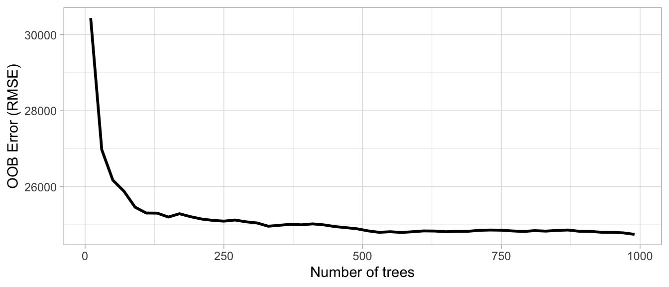
Figure 11.1: The Ames data has 80 features and starting with 10 times the number of features typically ensures the error estimate converges.

11.4.2 \(m_{try}\)

The hyperparameter that controls the split-variable randomization feature of random forests is often referred to as \(m_{try}\) and it helps to balance low tree correlation with reasonable predictive strength. With regression problems the default value is often \(m_{try} = \frac{p}{3}\) and for classification \(m_{try} = \sqrt{p}\). However, when there are fewer relevant predictors (e.g., noisy data) a higher value of \(m_{try}\) tends to perform better because it makes it more likely to select those features with the strongest signal. When there are many relevant predictors, a lower \(m_{try}\) might perform better.

Start with five evenly spaced values of \(m_{try}\) across the range 2–\(p\) centered at the recommended default as illustrated in Figure 11.2.

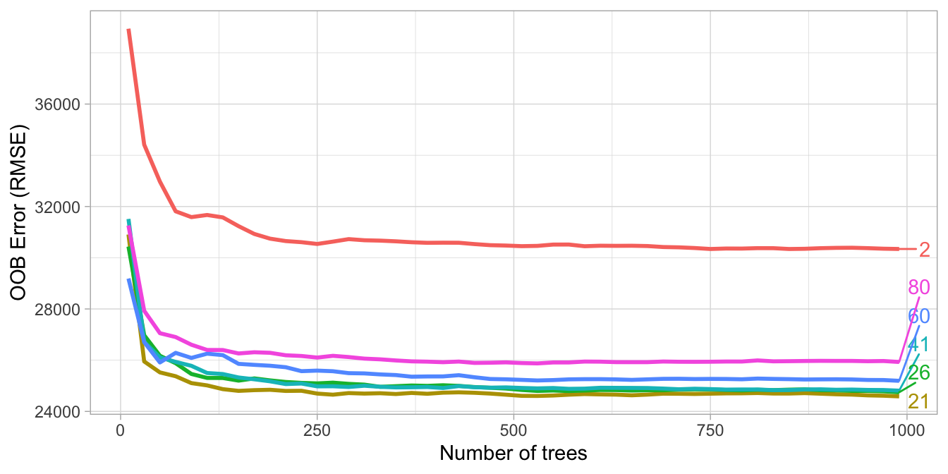
Figure 11.2: For the Ames data, an mtry value slightly lower (21) than the default (26) improves performance.

11.4.3 Tree complexity

Random forests are built on individual decision trees; consequently, most random forest implementations have one or more hyperparameters that allow us to control the depth and complexity of the individual trees. This will often include hyperparameters such as node size, max depth, max number of terminal nodes, or the required node size to allow additional splits. Node size is probably the most common hyperparameter to control tree complexity and most implementations use the default values of one for classification and five for regression as these values tend to produce good results (Dı'az-Uriarte and De Andres 2006; Goldstein, Polley, and Briggs 2011). However, Segal (2004) showed that if your data has many noisy predictors and higher \(m_{try}\) values are performing best, then performance may improve by increasing node size (i.e., decreasing tree depth and complexity). Moreover, if computation time is a concern then you can often decrease run time substantially by increasing the node size and have only marginal impacts to your error estimate as illustrated in Figure 11.3.

When adjusting node size start with three values between 1–10 and adjust depending on impact to accuracy and run time.

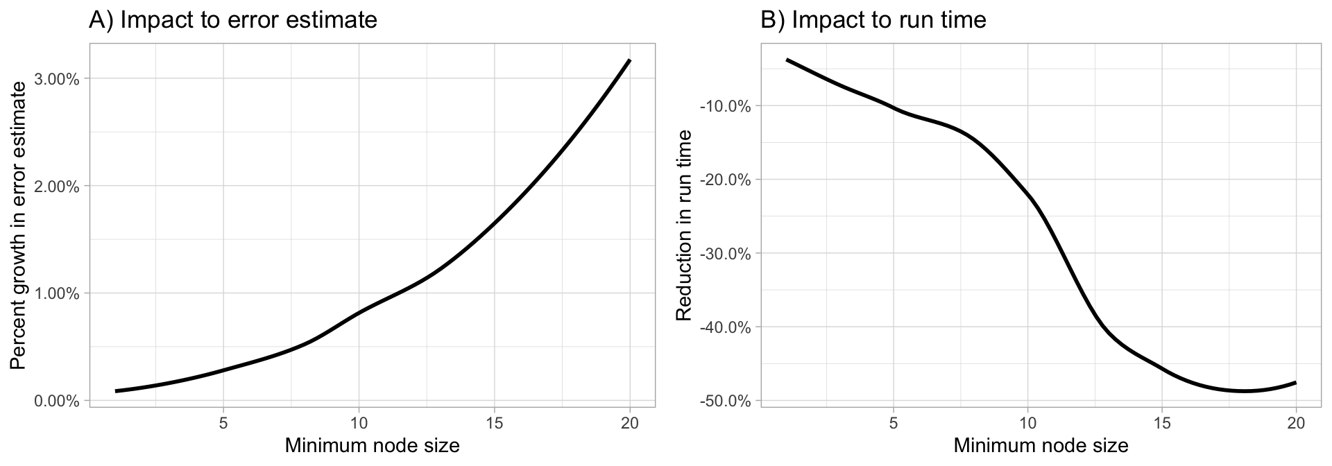
Figure 11.3: Increasing node size to reduce tree complexity will often have a larger impact on computation speed (right) than on your error estimate.

11.4.4 Sampling scheme

The default sampling scheme for random forests is bootstrapping where 100% of the observations are sampled with replacement (in other words, each bootstrap copy has the same size as the original training data); however, we can adjust both the sample size and whether to sample with or without replacement. The sample size parameter determines how many observations are drawn for the training of each tree. Decreasing the sample size leads to more diverse trees and thereby lower between-tree correlation, which can have a positive effect on the prediction accuracy. Consequently, if there are a few dominating features in your data set, reducing the sample size can also help to minimize between-tree correlation.

Also, when you have many categorical features with a varying number of levels, sampling with replacement can lead to biased variable split selection (Janitza, Binder, and Boulesteix 2016; Strobl et al. 2007). Consequently, if you have categories that are not balanced, sampling without replacement provides a less biased use of all levels across the trees in the random forest.

Assess 3–4 values of sample sizes ranging from 25%–100% and if you have unbalanced categorical features try sampling without replacement.

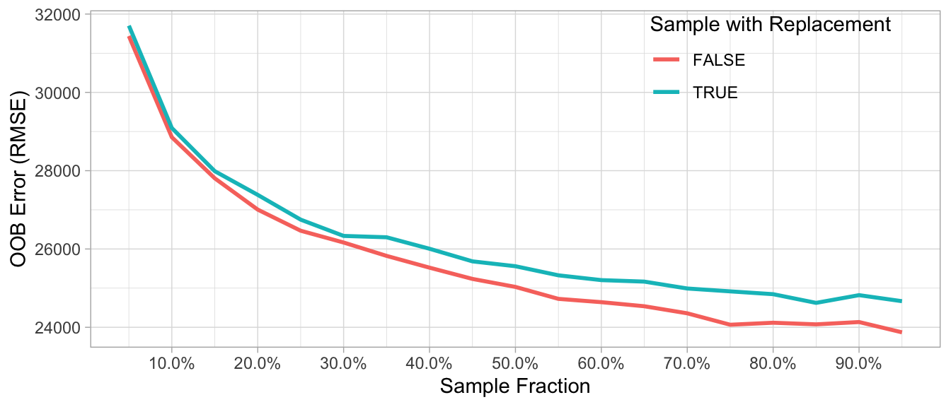
Figure 11.4: The Ames data has several imbalanced categorical features such as neighborhood, zoning, overall quality, and more. Consequently, sampling without replacement appears to improve performance as it leads to less biased split variable selection and more uncorrelated trees.

11.4.5 Split rule

Recall the default splitting rule during random forests tree building consists of selecting, out of all splits of the (randomly selected \(m_{try}\)) candidate variables, the split that minimizes the Gini impurity (in the case of classification) and the SSE (in case of regression). However, Strobl et al. (2007) illustrated that these default splitting rules favor the selection of features with many possible splits (e.g., continuous variables or categorical variables with many categories) over variables with fewer splits (the extreme case being binary variables, which have only one possible split). Conditional inference trees (Hothorn, Hornik, and Zeileis 2006) implement an alternative splitting mechanism that helps to reduce this variable selection bias.³¹ However, ensembling conditional inference trees has yet to be proven superior with regards to predictive accuracy and they take a lot longer to train.

To increase computational efficiency, splitting rules can be randomized where only a random subset of possible splitting values is considered for a variable (Geurts, Ernst, and Wehenkel 2006). If only a single random splitting value is randomly selected then we call this procedure extremely randomized trees. Due to the added randomness of split points, this method tends to have no improvement, or often a negative impact, on predictive accuracy.

Regarding runtime, extremely randomized trees are the fastest as the cutpoints are drawn completely randomly, followed by the classical random forest, while for conditional inference forests the runtime is the largest (Probst, Wright, and Boulesteix 2019).

If you need to increase computation time significantly try completely randomized trees; however, be sure to assess predictive accuracy to traditional split rules as this approach often has a negative impact on your loss function.

11.5 Tuning strategies

As we introduce more complex algorithms with greater number of hyperparameters, we should become more strategic with our tuning strategies. One way to become more strategic is to consider how we proceed through our grid search. Up to this point, all our grid searches have been full Cartesian grid searches where we assess every combination of hyperparameters of interest. We could continue to do the same; for example, the next code block searches across 120 combinations of hyperparameter settings.

This grid search takes approximately 2 minutes.

# create hyperparameter grid
hyper_grid <- expand.grid(
  mtry = floor(n_features * c(.05, .15, .25, .333, .4)),
  min.node.size = c(1, 3, 5, 10), 
  replace = c(TRUE, FALSE),                               
  sample.fraction = c(.5, .63, .8),                       
  rmse = NA                                               
)

# execute full cartesian grid search
for(i in seq_len(nrow(hyper_grid))) {
  # fit model for ith hyperparameter combination
  fit <- ranger(
    formula         = Sale_Price ~ ., 
    data            = ames_train, 
    num.trees       = n_features * 10,
    mtry            = hyper_grid$mtry[i],
    min.node.size   = hyper_grid$min.node.size[i],
    replace         = hyper_grid$replace[i],
    sample.fraction = hyper_grid$sample.fraction[i],
    verbose         = FALSE,
    seed            = 123,
    respect.unordered.factors = 'order',
  )
  # export OOB error 
  hyper_grid$rmse[i] <- sqrt(fit$prediction.error)
}

# assess top 10 models
hyper_grid %>%
  arrange(rmse) %>%
  mutate(perc_gain = (default_rmse - rmse) / default_rmse * 100) %>%
  head(10)
##    mtry min.node.size replace sample.fraction     rmse perc_gain
## 1    32             1   FALSE             0.8 23975.32  3.555819
## 2    32             3   FALSE             0.8 24022.97  3.364127
## 3    32             5   FALSE             0.8 24032.69  3.325041
## 4    26             3   FALSE             0.8 24103.53  3.040058
## 5    20             1   FALSE             0.8 24132.35  2.924142
## 6    26             5   FALSE             0.8 24144.38  2.875752
## 7    20             3   FALSE             0.8 24194.64  2.673560
## 8    26             1   FALSE             0.8 24216.02  2.587589
## 9    32            10   FALSE             0.8 24224.18  2.554755
## 10   20             5   FALSE             0.8 24249.46  2.453056

If we look at the results we see that the top 10 models are all near or below an RMSE of 24000 (a 2.5%–3.5% improvement over our baseline model). In these results, the default mtry value of \(\left \lfloor{\frac{\texttt{# features}}{3}}\right \rfloor = 26\) is nearly sufficient and smaller node sizes (deeper trees) perform best. What stands out the most is that taking less than 100% sample rate and sampling without replacement consistently performs best. Sampling less than 100% adds additional randomness in the procedure, which helps to further de-correlate the trees. Sampling without replacement likely improves performance because this data has a lot of high cardinality categorical features that are imbalanced.

However, as we add more hyperparameters and values to search across and as our data sets become larger, you can see how a full Cartesian search can become exhaustive and computationally expensive. In addition to full Cartesian search, the h2o package provides a random grid search that allows you to jump from one random combination to another and it also provides early stopping rules that allow you to stop the grid search once a certain condition is met (e.g., a certain number of models have been trained, a certain runtime has elapsed, or the accuracy has stopped improving by a certain amount). Although using a random discrete search path will likely not find the optimal model, it typically does a good job of finding a very good model.

To fit a random forest model with h2o, we first need to initiate our h2o session.

h2o.no_progress()
h2o.init(max_mem_size = "5g")

Next, we need to convert our training and test data sets to objects that h2o can work with.

# convert training data to h2o object
train_h2o <- as.h2o(ames_train)

# set the response column to Sale_Price
response <- "Sale_Price"

# set the predictor names
predictors <- setdiff(colnames(ames_train), response)

The following fits a default random forest model with h2o to illustrate that our baseline results (\(\text{OOB RMSE} = 24439\)) are very similar to the baseline ranger model we fit earlier.

h2o_rf1 <- h2o.randomForest(
    x = predictors, 
    y = response,
    training_frame = train_h2o, 
    ntrees = n_features * 10,
    seed = 123
)

h2o_rf1
## Model Details:
## ==============
## 
## H2ORegressionModel: drf
## Model ID:  DRF_model_R_1554292876245_2 
## Model Summary: 
##   number_of_trees number_of_internal_trees model_size_in_bytes min_depth max_depth mean_depth min_leaves max_leaves mean_leaves
## 1             800                      800            12365675        19        20   19.99875       1148       1283  1225.04630
## 
## 
## H2ORegressionMetrics: drf
## ** Reported on training data. **
## ** Metrics reported on Out-Of-Bag training samples **
## 
## MSE:  597254712
## RMSE:  24438.8
## MAE:  14833.34
## RMSLE:  0.1396219
## Mean Residual Deviance :  597254712

To execute a grid search in h2o we need our hyperparameter grid to be a list. For example, the following code searches a larger grid space than before with a total of 240 hyperparameter combinations. We then create a random grid search strategy that will stop if none of the last 10 models have managed to have a 0.1% improvement in MSE compared to the best model before that. If we continue to find improvements then we cut the grid search off after 300 seconds (5 minutes).

# hyperparameter grid
hyper_grid <- list(
  mtries = floor(n_features * c(.05, .15, .25, .333, .4)),
  min_rows = c(1, 3, 5, 10),
  max_depth = c(10, 20, 30),
  sample_rate = c(.55, .632, .70, .80)
)

# random grid search strategy
search_criteria <- list(
  strategy = "RandomDiscrete",
  stopping_metric = "mse",
  stopping_tolerance = 0.001,   # stop if improvement is < 0.1%
  stopping_rounds = 10,         # over the last 10 models
  max_runtime_secs = 60*5      # or stop search after 5 min.
)

We can then perform the grid search with h2o.grid(). The following executes the grid search with early stopping turned on. The early stopping we specify below in h2o.grid() will stop growing an individual random forest model if we have not experienced at least a 0.05% improvement in the overall OOB error in the last 10 trees. This is very useful as we can specify to build 1000 trees for each random forest model but h2o may only build 200 trees if we don’t experience any improvement.

This grid search takes 5 minutes.

# perform grid search 
random_grid <- h2o.grid(
  algorithm = "randomForest",
  grid_id = "rf_random_grid",
  x = predictors, 
  y = response, 
  training_frame = train_h2o,
  hyper_params = hyper_grid,
  ntrees = n_features * 10,
  seed = 123,
  stopping_metric = "RMSE",   
  stopping_rounds = 10,           # stop if last 10 trees added 
  stopping_tolerance = 0.005,     # don't improve RMSE by 0.5%
  search_criteria = search_criteria
)

Our grid search assessed 129 models before stopping due to time. The best model (max_depth = 30, min_rows = 1, mtries = 20, and sample_rate = 0.8) achieved an OOB RMSE of 23932. So although our random search assessed about 30% of the number of models as a full grid search would, the more efficient random search found a near-optimal model within the specified time constraint.

In fact, we re-ran the same grid search but allowed for a full search across all 240 hyperparameter combinations and the best model achieved an OOB RMSE of 23785.

# collect the results and sort by our model performance metric 
# of choice
random_grid_perf <- h2o.getGrid(
  grid_id = "rf_random_grid", 
  sort_by = "mse", 
  decreasing = FALSE
)
random_grid_perf
## H2O Grid Details
## ================
## 
## Grid ID: rf_random_grid 
## Used hyper parameters: 
##   -  max_depth 
##   -  min_rows 
##   -  mtries 
##   -  sample_rate 
## Number of models: 129 
## Number of failed models: 0 
## 
## Hyper-Parameter Search Summary: ordered by increasing mse
##   max_depth min_rows mtries sample_rate                 model_ids                 mse
## 1        30      1.0     20         0.8  rf_random_grid_model_113 5.727214331253618E8
## 2        20      1.0     20         0.8   rf_random_grid_model_39 5.727741137204964E8
## 3        20      1.0     32         0.7    rf_random_grid_model_8  5.76799145123527E8
## 4        30      1.0     26         0.7   rf_random_grid_model_67 5.815643260591004E8
## 5        30      1.0     12         0.8   rf_random_grid_model_64 5.951710701891141E8
## 
## ---
##     max_depth min_rows mtries sample_rate                model_ids                  mse
## 124        10     10.0      4         0.7  rf_random_grid_model_44 1.0367731339073703E9
## 125        20     10.0      4         0.8  rf_random_grid_model_73 1.0451421787520385E9
## 126        20      5.0      4        0.55  rf_random_grid_model_12 1.0710840266353173E9
## 127        10      5.0      4        0.55  rf_random_grid_model_75 1.0793293549247448E9
## 128        10     10.0      4       0.632  rf_random_grid_model_37 1.0804801985871077E9
## 129        20     10.0      4        0.55  rf_random_grid_model_22 1.1525799087784908E9

11.6 Feature interpretation

Computing feature importance and feature effects for random forests follow the same procedure as discussed in Section 10.5. However, in addition to the impurity-based measure of feature importance where we base feature importance on the average total reduction of the loss function for a given feature across all trees, random forests also typically include a permutation-based importance measure. In the permutation-based approach, for each tree, the OOB sample is passed down the tree and the prediction accuracy is recorded. Then the values for each variable (one at a time) are randomly permuted and the accuracy is again computed. The decrease in accuracy as a result of this randomly shuffling of feature values is averaged over all the trees for each predictor. The variables with the largest average decrease in accuracy are considered most important.

For example, we can compute both measures of feature importance with ranger by setting the importance argument.

For ranger, once you’ve identified the optimal parameter values from the grid search, you will want to re-run your model with these hyperparameter values. You can also crank up the number of trees, which will help create more stables values of variable importance.

# re-run model with impurity-based variable importance
rf_impurity <- ranger(
  formula = Sale_Price ~ ., 
  data = ames_train, 
  num.trees = 2000,
  mtry = 32,
  min.node.size = 1,
  sample.fraction = .80,
  replace = FALSE,
  importance = "impurity",
  respect.unordered.factors = "order",
  verbose = FALSE,
  seed  = 123
)

# re-run model with permutation-based variable importance
rf_permutation <- ranger(
  formula = Sale_Price ~ ., 
  data = ames_train, 
  num.trees = 2000,
  mtry = 32,
  min.node.size = 1,
  sample.fraction = .80,
  replace = FALSE,
  importance = "permutation",
  respect.unordered.factors = "order",
  verbose = FALSE,
  seed  = 123
)

The resulting VIPs are displayed in Figure 11.5. Typically, you will not see the same variable importance order between the two options; however, you will often see similar variables at the top of the plots (and also the bottom). Consequently, in this example, we can comfortably state that there appears to be enough evidence to suggest that three variables stand out as most influential:

• Overall_Qual
  
• Gr_Liv_Area
  
• Neighborhood

Looking at the next ~10 variables in both plots, you will also see some commonality in influential variables (e.g., Garage_Cars, Exter_Qual, Bsmt_Qual, and Year_Built).

p1 <- vip::vip(rf_impurity, num_features = 25, bar = FALSE)
p2 <- vip::vip(rf_permutation, num_features = 25, bar = FALSE)

gridExtra::grid.arrange(p1, p2, nrow = 1)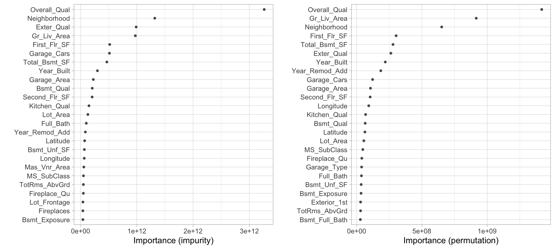

Figure 11.5: Top 25 most important variables based on impurity (left) and permutation (right).

11.7 Final thoughts

Random forests provide a very powerful out-of-the-box algorithm that often has great predictive accuracy. They come with all the benefits of decision trees (with the exception of surrogate splits) and bagging but greatly reduce instability and between-tree correlation. And due to the added split variable selection attribute, random forests are also faster than bagging as they have a smaller feature search space at each tree split. However, random forests will still suffer from slow computational speed as your data sets get larger but, similar to bagging, the algorithm is built upon independent steps, and most modern implementations (e.g., ranger, h2o) allow for parallelization to improve training time.

References

Breiman, Leo. 2001. “Random Forests.” Machine Learning 45 (1). Springer: 5–32.

Dı'az-Uriarte, Ramón, and Sara Alvarez De Andres. 2006. “Gene Selection and Classification of Microarray Data Using Random Forest.” BMC Bioinformatics 7 (1). BioMed Central: 3.

Friedman, Jerome, Trevor Hastie, and Robert Tibshirani. 2001. The Elements of Statistical Learning. Vol. 1. Springer Series in Statistics New York, NY, USA:

Geurts, Pierre, Damien Ernst, and Louis Wehenkel. 2006. “Extremely Randomized Trees.” Machine Learning 63 (1). Springer: 3–42.

Goldstein, Benjamin A, Eric C Polley, and Farren BS Briggs. 2011. “Random Forests for Genetic Association Studies.” Statistical Applications in Genetics and Molecular Biology 10 (1). De Gruyter.

Hothorn, Torsten, Kurt Hornik, and Achim Zeileis. 2006. “Unbiased Recursive Partitioning: A Conditional Inference Framework.” Journal of Computational and Graphical Statistics 15 (3). Taylor & Francis: 651–74.

Janitza, Silke, Harald Binder, and Anne-Laure Boulesteix. 2016. “Pitfalls of Hypothesis Tests and Model Selection on Bootstrap Samples: Causes and Consequences in Biometrical Applications.” Biometrical Journal 58 (3). Wiley Online Library: 447–73.

Probst, Philipp, Bernd Bischl, and Anne-Laure Boulesteix. 2018. “Tunability: Importance of Hyperparameters of Machine Learning Algorithms.” arXiv Preprint arXiv:1802.09596.

Probst, Philipp, Marvin N Wright, and Anne-Laure Boulesteix. 2019. “Hyperparameters and Tuning Strategies for Random Forest.” Wiley Interdisciplinary Reviews: Data Mining and Knowledge Discovery. Wiley Online Library, e1301.

Segal, Mark R. 2004. “Machine Learning Benchmarks and Random Forest Regression.” UCSF: Center for Bioinformatics and Molecular Biostatistics.

Strobl, Carolin, Anne-Laure Boulesteix, Achim Zeileis, and Torsten Hothorn. 2007. “Bias in Random Forest Variable Importance Measures: Illustrations, Sources and a Solution.” BMC Bioinformatics 8 (1). BioMed Central: 25.

Wright, Marvin, and Andreas Ziegler. 2017. “Ranger: A Fast Implementation of Random Forests for High Dimensional Data in C++ and R.” Journal of Statistical Software, Articles 77 (1): 1–17. https://doi.org/10.18637/jss.v077.i01.

---

29. See J. Friedman, Hastie, and Tibshirani (2001) for a mathematical explanation of the tree correlation phenomenon.↩

30. Here we use the ranger package to fit a baseline random forest. It is common for folks to first learn to implement random forests by using the original randomForest package (Liaw and Wiener 2002). Although randomForest is a great package with many bells and whistles, ranger provides a much faster C++ implementation of the same algorithm.↩

31. Conditional inference trees are available in the partykit (Hothorn and Zeileis 2015) and ranger packages among others.↩