Chapter 4 Linear Regression

Linear regression, a staple of classical statistical modeling, is one of the simplest algorithms for doing supervised learning. Though it may seem somewhat dull compared to some of the more modern statistical learning approaches described in later chapters, linear regression is still a useful and widely applied statistical learning method. Moreover, it serves as a good starting point for more advanced approaches; as we will see in later chapters, many of the more sophisticated statistical learning approaches can be seen as generalizations to or extensions of ordinary linear regression. Consequently, it is important to have a good understanding of linear regression before studying more complex learning methods. This chapter introduces linear regression with an emphasis on prediction, rather than inference. An excellent and comprehensive overview of linear regression is provided in Kutner et al. (2005). See Faraway (2016b) for a discussion of linear regression in R (the book’s website also provides Python scripts).

4.1 Prerequisites

This chapter leverages the following packages:

# Helper packages
library(dplyr)    # for data manipulation
library(ggplot2)  # for awesome graphics

# Modeling packages
library(caret)    # for cross-validation, etc.

# Model interpretability packages
library(vip)      # variable importance

We’ll also continue working with the ames_train data set created in Section 2.7.

4.2 Simple linear regression

Pearson’s correlation coefficient is often used to quantify the strength of the linear association between two continuous variables. In this section, we seek to fully characterize that linear relationship. Simple linear regression (SLR) assumes that the statistical relationship between two continuous variables (say \(X\) and \(Y\)) is (at least approximately) linear:

\[\begin{equation} \tag{4.1} Y_i = \beta_0 + \beta_1 X_i + \epsilon_i, \quad \text{for } i = 1, 2, \dots, n, \end{equation}\]

where \(Y_i\) represents the i-th response value, \(X_i\) represents the i-th feature value, \(\beta_0\) and \(\beta_1\) are fixed, but unknown constants (commonly referred to as coefficients or parameters) that represent the intercept and slope of the regression line, respectively, and \(\epsilon_i\) represents noise or random error. In this chapter, we’ll assume that the errors are normally distributed with mean zero and constant variance \(\sigma^2\), denoted \(\stackrel{iid}{\sim} \left(0, \sigma^2\right)\). Since the random errors are centered around zero (i.e., \(E\left(\epsilon\right) = 0\)), linear regression is really a problem of estimating a conditional mean:

\[\begin{equation} E\left(Y_i | X_i\right) = \beta_0 + \beta_1 X_i. \end{equation}\]

For brevity, we often drop the conditional piece and write \(E\left(Y | X\right) = E\left(Y\right)\). Consequently, the interpretation of the coefficients is in terms of the average, or mean response. For example, the intercept \(\beta_0\) represents the average response value when \(X = 0\) (it is often not meaningful or of interest and is sometimes referred to as a bias term). The slope \(\beta_1\) represents the increase in the average response per one-unit increase in \(X\) (i.e., it is a rate of change).

4.2.1 Estimation

Ideally, we want estimates of \(\beta_0\) and \(\beta_1\) that give us the “best fitting” line. But what is meant by “best fitting”? The most common approach is to use the method of least squares (LS) estimation; this form of linear regression is often referred to as ordinary least squares (OLS) regression. There are multiple ways to measure “best fitting”, but the LS criterion finds the “best fitting” line by minimizing the residual sum of squares (RSS):

\[\begin{equation} \tag{4.2} RSS\left(\beta_0, \beta_1\right) = \sum_{i=1}^n\left[Y_i - \left(\beta_0 + \beta_1 X_i\right)\right]^2 = \sum_{i=1}^n\left(Y_i - \beta_0 - \beta_1 X_i\right)^2. \end{equation}\]

The LS estimates of \(\beta_0\) and \(\beta_1\) are denoted as \(\widehat{\beta}_0\) and \(\widehat{\beta}_1\), respectively. Once obtained, we can generate predicted values, say at \(X = X_{new}\), using the estimated regression equation:

\[\begin{equation} \widehat{Y}_{new} = \widehat{\beta}_0 + \widehat{\beta}_1 X_{new}, \end{equation}\]

where \(\widehat{Y}_{new} = \widehat{E\left(Y_{new} | X = X_{new}\right)}\) is the estimated mean response at \(X = X_{new}\).

With the Ames housing data, suppose we wanted to model a linear relationship between the total above ground living space of a home (Gr_Liv_Area) and sale price (Sale_Price). To perform an OLS regression model in R we can use the lm() function:

model1 <- lm(Sale_Price ~ Gr_Liv_Area, data = ames_train)

The fitted model (model1) is displayed in the left plot in Figure 4.1 where the points represent the values of Sale_Price in the training data. In the right plot of Figure 4.1, the vertical lines represent the individual errors, called residuals, associated with each observation. The OLS criterion in Equation (4.2) identifies the “best fitting” line that minimizes the sum of squares of these residuals.

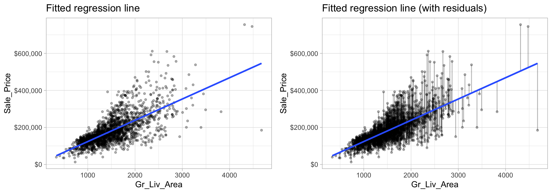
Figure 4.1: The least squares fit from regressing sale price on living space for the the Ames housing data. Left: Fitted regression line. Right: Fitted regression line with vertical grey bars representing the residuals.

The coef() function extracts the estimated coefficients from the model. We can also use summary() to get a more detailed report of the model results.

summary(model1) 
## 
## Call:
## lm(formula = Sale_Price ~ Gr_Liv_Area, data = ames_train)
## 
## Residuals:
##     Min      1Q  Median      3Q     Max 
## -361143  -30668   -2449   22838  331357 
## 
## Coefficients:
##             Estimate Std. Error t value            Pr(>|t|)    
## (Intercept) 8732.938   3996.613   2.185               0.029 *  
## Gr_Liv_Area  114.876      2.531  45.385 <0.0000000000000002 ***
## ---
## Signif. codes:  0 '***' 0.001 '**' 0.01 '*' 0.05 '.' 0.1 ' ' 1
## 
## Residual standard error: 56700 on 2051 degrees of freedom
## Multiple R-squared:  0.5011, Adjusted R-squared:  0.5008 
## F-statistic:  2060 on 1 and 2051 DF,  p-value: < 0.00000000000000022

The estimated coefficients from our model are \(\widehat{\beta}_0 =\) 8732.94 and \(\widehat{\beta}_1 =\) 114.88. To interpret, we estimate that the mean selling price increases by 114.88 for each additional one square foot of above ground living space. This simple description of the relationship between the sale price and square footage using a single number (i.e., the slope) is what makes linear regression such an intuitive and popular modeling tool.

One drawback of the LS procedure in linear regression is that it only provides estimates of the coefficients; it does not provide an estimate of the error variance \(\sigma^2\)! LS also makes no assumptions about the random errors. These assumptions are important for inference and in estimating the error variance which we’re assuming is a constant value \(\sigma^2\). One way to estimate \(\sigma^2\) (which is required for characterizing the variability of our fitted model), is to use the method of maximum likelihood (ML) estimation (see Kutner et al. (2005) Section 1.7 for details). The ML procedure requires that we assume a particular distribution for the random errors. Most often, we assume the errors to be normally distributed. In practice, under the usual assumptions stated above, an unbiased estimate of the error variance is given as the sum of the squared residuals divided by \(n - p\) (where \(p\) is the number of regression coefficients or parameters in the model):

\[\begin{equation} \widehat{\sigma}^2 = \frac{1}{n - p}\sum_{i = 1} ^ n r_i ^ 2, \end{equation}\]

where \(r_i = \left(Y_i - \widehat{Y}_i\right)\) is referred to as the \(i\)th residual (i.e., the difference between the \(i\)th observed and predicted response value). The quantity \(\widehat{\sigma}^2\) is also referred to as the mean square error (MSE) and its square root is denoted RMSE (see Section 2.6 for discussion on these metrics). In R, the RMSE of a linear model can be extracted using the sigma() function:

Typically, these error metrics are computed on a separate validation set or using cross-validation as discussed in Section 2.4; however, they can also be computed on the same training data the model was trained on as illustrated here.

sigma(model1)    # RMSE
## [1] 56704.78
sigma(model1)^2  # MSE
## [1] 3215432370

Note that the RMSE is also reported as the Residual standard error in the output from summary().

4.2.2 Inference

How accurate are the LS of \(\beta_0\) and \(\beta_1\)? Point estimates by themselves are not very useful. It is often desirable to associate some measure of an estimates variability. The variability of an estimate is often measured by its standard error (SE)—the square root of its variance. If we assume that the errors in the linear regression model are \(\stackrel{iid}{\sim} \left(0, \sigma^2\right)\), then simple expressions for the SEs of the estimated coefficients exist and are displayed in the column labeled Std. Error in the output from summary(). From this, we can also derive simple \(t\)-tests to understand if the individual coefficients are statistically significant from zero. The t-statistics for such a test are nothing more than the estimated coefficients divided by their corresponding estimated standard errors (i.e., in the output from summary(), t value = Estimate / Std. Error). The reported t-statistics measure the number of standard deviations each coefficient is away from 0. Thus, large t-statistics (greater than two in absolute value, say) roughly indicate statistical significance at the \(\alpha = 0.05\) level. The p-values for these tests are also reported by summary() in the column labeled Pr(>|t|).

Under the same assumptions, we can also derive confidence intervals for the coefficients. The formula for the traditional \(100\left(1 - \alpha\right)\)% confidence interval for \(\beta_j\) is

\[\begin{equation} \widehat{\beta}_j \pm t_{1 - \alpha / 2, n - p} \widehat{SE}\left(\widehat{\beta}_j\right). \tag{4.3} \end{equation}\]

In R, we can construct such (one-at-a-time) confidence intervals for each coefficient using confint(). For example, a 95% confidence intervals for the coefficients in our SLR example can be computed using

confint(model1, level = 0.95)
##                2.5 %     97.5 %
## (Intercept) 895.0961 16570.7805
## Gr_Liv_Area 109.9121   119.8399

To interpret, we estimate with 95% confidence that the mean selling price increases between 109.91 and 119.84 for each additional one square foot of above ground living space. We can also conclude that the slope \(\beta_1\) is significantly different from zero (or any other pre-specified value not included in the interval) at the \(\alpha = 0.05\) level. This is also supported by the output from summary().

Most statistical software, including R, will include estimated standard errors, t-statistics, etc. as part of its regression output. However, it is important to remember that such quantities depend on three major assumptions of the linear regression model:

1. Independent observations
2. The random errors have mean zero, and constant variance
3. The random errors are normally distributed

If any or all of these assumptions are violated, then remedial measures need to be taken. For instance, weighted least squares (and other procedures) can be used when the constant variance assumption is violated. Transformations (of both the response and features) can also help to correct departures from these assumptions. The residuals are extremely useful in helping to identify how parametric models depart from such assumptions.

4.3 Multiple linear regression

In practice, we often have more than one predictor. For example, with the Ames housing data, we may wish to understand if above ground square footage (Gr_Liv_Area) and the year the house was built (Year_Built) are (linearly) related to sale price (Sale_Price). We can extend the SLR model so that it can directly accommodate multiple predictors; this is referred to as the multiple linear regression (MLR) model. With two predictors, the MLR model becomes:

\[\begin{equation} Y = \beta_0 + \beta_1 X_1 + \beta_2 X_2 + \epsilon, \end{equation}\]

where \(X_1\) and \(X_2\) are features of interest. In our Ames housing example, \(X_1\) represents Gr_Liv_Area and \(X_2\) represents Year_Built.

In R, multiple linear regression models can be fit by separating all the features of interest with a +:

(model2 <- lm(Sale_Price ~ Gr_Liv_Area + Year_Built, data = ames_train))
## 
## Call:
## lm(formula = Sale_Price ~ Gr_Liv_Area + Year_Built, data = ames_train)
## 
## Coefficients:
## (Intercept)  Gr_Liv_Area   Year_Built  
## -2123054.21        99.18      1093.48

Alternatively, we can use update() to update the model formula used in model1. The new formula can use a . as shorthand for keep everything on either the left or right hand side of the formula, and a + or - can be used to add or remove terms from the original model, respectively. In the case of adding Year_Built to model1, we could’ve used:

(model2 <- update(model1, . ~ . + Year_Built))
## 
## Call:
## lm(formula = Sale_Price ~ Gr_Liv_Area + Year_Built, data = ames_train)
## 
## Coefficients:
## (Intercept)  Gr_Liv_Area   Year_Built  
## -2123054.21        99.18      1093.48

The LS estimates of the regression coefficients are \(\widehat{\beta}_1 =\) 99.176 and \(\widehat{\beta}_2 =\) 1093.485 (the estimated intercept is -2123054.207. In other words, every one square foot increase to above ground square footage is associated with an additional $99.18 in mean selling price when holding the year the house was built constant. Likewise, for every year newer a home is there is approximately an increase of $1,093.48 in selling price when holding the above ground square footage constant.

A contour plot of the fitted regression surface is displayed in the left side of Figure 4.2 below. Note how the fitted regression surface is flat (i.e., it does not twist or bend). This is true for all linear models that include only main effects (i.e., terms involving only a single predictor). One way to model curvature is to include interaction effects. An interaction occurs when the effect of one predictor on the response depends on the values of other predictors. In linear regression, interactions can be captured via products of features (i.e., \(X_1 \times X_2\)). A model with two main effects can also include a two-way interaction. For example, to include an interaction between \(X_1 =\) Gr_Liv_Area and \(X_2 =\) Year_Built, we introduce an additional product term:

\[\begin{equation} Y = \beta_0 + \beta_1 X_1 + \beta_2 X_2 + \beta_3 X_1 X_2 + \epsilon. \end{equation}\]

Note that in R, we use the : operator to include an interaction (technically, we could use * as well, but x1 * x2 is shorthand for x1 + x2 + x1:x2 so is slightly redundant):

lm(Sale_Price ~ Gr_Liv_Area + Year_Built + Gr_Liv_Area:Year_Built, data = ames_train)
## 
## Call:
## lm(formula = Sale_Price ~ Gr_Liv_Area + Year_Built + Gr_Liv_Area:Year_Built, 
##     data = ames_train)
## 
## Coefficients:
##            (Intercept)             Gr_Liv_Area              Year_Built  
##            382194.3015              -1483.8810               -179.7979  
## Gr_Liv_Area:Year_Built  
##                 0.8037

A contour plot of the fitted regression surface with interaction is displayed in the right side of Figure 4.2. Note the curvature in the contour lines.

Interaction effects are quite prevalent in predictive modeling. Since linear models are an example of parametric modeling, it is up to the analyst to decide if and when to include interaction effects. In later chapters, we’ll discuss algorithms that can automatically detect and incorporate interaction effects (albeit in different ways). It is also important to understand a concept called the hierarchy principle—which demands that all lower-order terms corresponding to an interaction be retained in the model—when considering interaction effects in linear regression models.

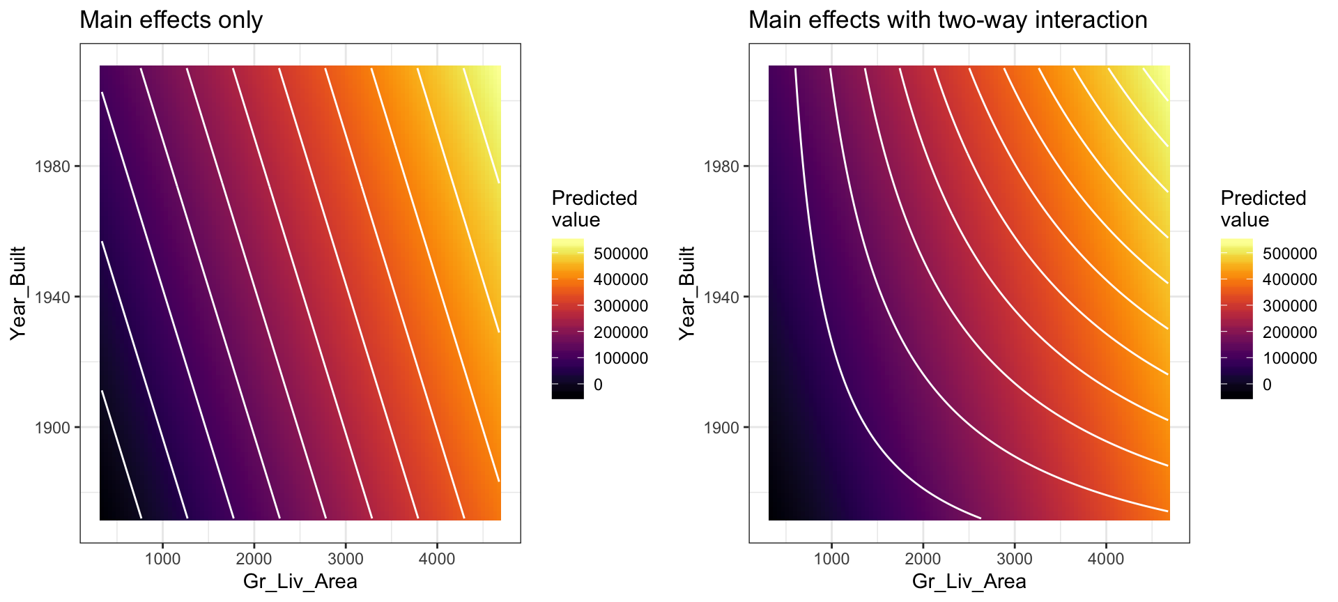
Figure 4.2: In a three-dimensional setting, with two predictors and one response, the least squares regression line becomes a plane. The ‘best-fit’ plane minimizes the sum of squared errors between the actual sales price (individual dots) and the predicted sales price (plane).

In general, we can include as many predictors as we want, as long as we have more rows than parameters! The general multiple linear regression model with p distinct predictors is

\[\begin{equation} Y = \beta_0 + \beta_1 X_1 + \beta_2 X_2 + \cdots + \beta_p X_p + \epsilon, \end{equation}\]

where \(X_i\) for \(i = 1, 2, \dots, p\) are the predictors of interest. Note some of these may represent interactions (e.g., \(X_3 = X_1 \times X_2\)) between or transformations¹⁸ (e.g., \(X_4 = \sqrt{X_1}\)) of the original features. Unfortunately, visualizing beyond three dimensions is not practical as our best-fit plane becomes a hyperplane. However, the motivation remains the same where the best-fit hyperplane is identified by minimizing the RSS. The code below creates a third model where we use all features in our data set as main effects (i.e., no interaction terms) to predict Sale_Price.

# include all possible main effects
model3 <- lm(Sale_Price ~ ., data = ames_train) 

# print estimated coefficients in a tidy data frame
broom::tidy(model3)  
## # A tibble: 283 x 5
##    term                                estimate std.error statistic p.value
##    <chr>                                  <dbl>     <dbl>     <dbl>   <dbl>
##  1 (Intercept)                          -5.61e6 11261881.    -0.498   0.618
##  2 MS_SubClassOne_Story_1945_and_Older   3.56e3     3843.     0.926   0.355
##  3 MS_SubClassOne_Story_with_Finished…   1.28e4    12834.     0.997   0.319
##  4 MS_SubClassOne_and_Half_Story_Unfi…   8.73e3    12871.     0.678   0.498
##  5 MS_SubClassOne_and_Half_Story_Fini…   4.11e3     6226.     0.660   0.509
##  6 MS_SubClassTwo_Story_1946_and_Newer  -1.09e3     5790.    -0.189   0.850
##  7 MS_SubClassTwo_Story_1945_and_Older   7.14e3     6349.     1.12    0.261
##  8 MS_SubClassTwo_and_Half_Story_All_…  -1.39e4    11003.    -1.27    0.206
##  9 MS_SubClassSplit_or_Multilevel       -1.15e4    10512.    -1.09    0.276
## 10 MS_SubClassSplit_Foyer               -4.39e3     8057.    -0.545   0.586
## # … with 273 more rows

4.4 Assessing model accuracy

We’ve fit three main effects models to the Ames housing data: a single predictor, two predictors, and all possible predictors. But the question remains, which model is “best”? To answer this question we have to define what we mean by “best”. In our case, we’ll use the RMSE metric and cross-validation (Section 2.4) to determine the “best” model. We can use the caret::train() function to train a linear model (i.e., method = "lm") using cross-validation (or a variety of other validation methods). In practice, a number of factors should be considered in determining a “best” model (e.g., time constraints, model production cost, predictive accuracy, etc.). The benefit of caret is that it provides built-in cross-validation capabilities, whereas the lm() function does not¹⁹. The following code chunk uses caret::train() to refit model1 using 10-fold cross-validation:

# Train model using 10-fold cross-validation
set.seed(123)  # for reproducibility
(cv_model1 <- train(
  form = Sale_Price ~ Gr_Liv_Area, 
  data = ames_train, 
  method = "lm",
  trControl = trainControl(method = "cv", number = 10)
))
## Linear Regression 
## 
## 2053 samples
##    1 predictor
## 
## No pre-processing
## Resampling: Cross-Validated (10 fold) 
## Summary of sample sizes: 1846, 1848, 1848, 1848, 1848, 1848, ... 
## Resampling results:
## 
##   RMSE      Rsquared   MAE     
##   56410.89  0.5069425  39169.09
## 
## Tuning parameter 'intercept' was held constant at a value of TRUE

The resulting cross-validated RMSE is $56,410.89 (this is the average RMSE across the 10 CV folds). How should we interpret this? When applied to unseen data, the predictions this model makes are, on average, about $56,410.89 off from the actual sale price.

We can perform cross-validation on the other two models in a similar fashion, which we do in the code chunk below.

# model 2 CV
set.seed(123)
cv_model2 <- train(
  Sale_Price ~ Gr_Liv_Area + Year_Built, 
  data = ames_train, 
  method = "lm",
  trControl = trainControl(method = "cv", number = 10)
)

# model 3 CV
set.seed(123)
cv_model3 <- train(
  Sale_Price ~ ., 
  data = ames_train, 
  method = "lm",
  trControl = trainControl(method = "cv", number = 10)
)

# Extract out of sample performance measures
summary(resamples(list(
  model1 = cv_model1, 
  model2 = cv_model2, 
  model3 = cv_model3
)))
## 
## Call:
## summary.resamples(object = resamples(list(model1 = cv_model1, model2
##  = cv_model2, model3 = cv_model3)))
## 
## Models: model1, model2, model3 
## Number of resamples: 10 
## 
## MAE 
##            Min.  1st Qu.   Median     Mean  3rd Qu.     Max. NA's
## model1 34457.58 36323.74 38943.81 39169.09 41660.81 45005.17    0
## model2 28094.79 30594.47 31959.30 32246.86 34210.70 37441.82    0
## model3 12458.27 15420.10 16484.77 16258.84 17262.39 19029.29    0
## 
## RMSE 
##            Min.  1st Qu.   Median     Mean  3rd Qu.     Max. NA's
## model1 47211.34 52363.41 54948.96 56410.89 60672.31 67679.05    0
## model2 37698.17 42607.11 45407.14 46292.38 49668.59 54692.06    0
## model3 20844.33 22581.04 24947.45 26098.00 27695.65 39521.49    0
## 
## Rsquared 
##             Min.   1st Qu.    Median      Mean   3rd Qu.      Max. NA's
## model1 0.3598237 0.4550791 0.5289068 0.5069425 0.5619841 0.5965793    0
## model2 0.5714665 0.6392504 0.6800818 0.6703298 0.7067458 0.7348562    0
## model3 0.7869022 0.9018567 0.9104351 0.8949642 0.9166564 0.9303504    0

Extracting the results for each model, we see that by adding more information via more predictors, we are able to improve the out-of-sample cross validation performance metrics. Specifically, our cross-validated RMSE reduces from $46,292.38 (the model with two predictors) down to $26,098.00 (for our full model). In this case, the model with all possible main effects performs the “best” (compared with the other two).

4.5 Model concerns

As previously stated, linear regression has been a popular modeling tool due to the ease of interpreting the coefficients. However, linear regression makes several strong assumptions that are often violated as we include more predictors in our model. Violation of these assumptions can lead to flawed interpretation of the coefficients and prediction results.

1. Linear relationship: Linear regression assumes a linear relationship between the predictor and the response variable. However, as discussed in Chapter 3, non-linear relationships can be made linear (or near-linear) by applying transformations to the response and/or predictors. For example, Figure 4.3 illustrates the relationship between sale price and the year a home was built. The left plot illustrates the non-linear relationship that exists. However, we can achieve a near-linear relationship by log transforming sale price, although some non-linearity still exists for older homes.

p1 <- ggplot(ames_train, aes(Year_Built, Sale_Price)) + 
  geom_point(size = 1, alpha = .4) +
  geom_smooth(se = FALSE) +
  scale_y_continuous("Sale price", labels = scales::dollar) +
  xlab("Year built") +
  ggtitle(paste("Non-transformed variables with a\n",
                "non-linear relationship."))

p2 <- ggplot(ames_train, aes(Year_Built, Sale_Price)) + 
  geom_point(size = 1, alpha = .4) + 
  geom_smooth(method = "lm", se = FALSE) +
  scale_y_log10("Sale price", labels = scales::dollar, 
                breaks = seq(0, 400000, by = 100000)) +
  xlab("Year built") +
  ggtitle(paste("Transforming variables can provide a\n",
                "near-linear relationship."))

gridExtra::grid.arrange(p1, p2, nrow = 1)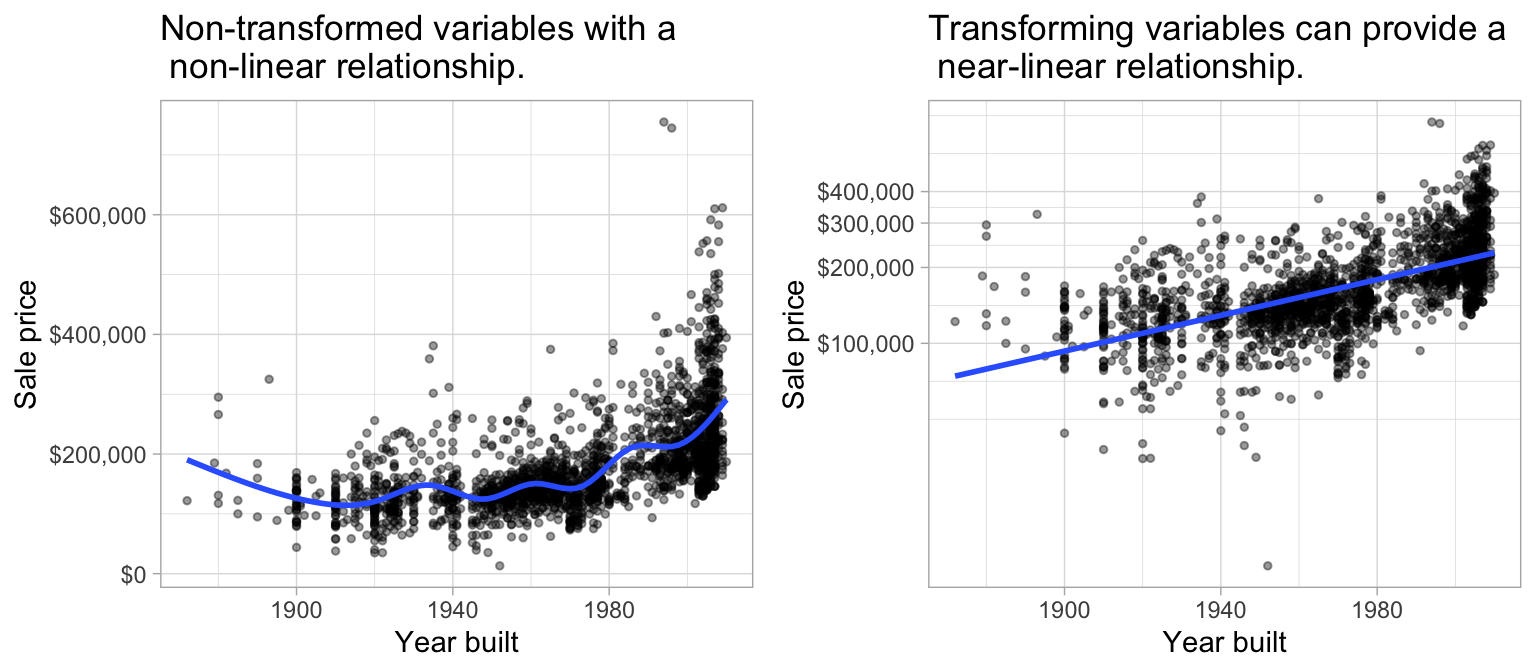

Figure 4.3: Linear regression assumes a linear relationship between the predictor(s) and the response variable; however, non-linear relationships can often be altered to be near-linear by applying a transformation to the variable(s).

2. Constant variance among residuals: Linear regression assumes the variance among error terms (\(\epsilon_1, \epsilon_2, \dots, \epsilon_p\)) are constant (this assumption is referred to as homoscedasticity). If the error variance is not constant, the p-values and confidence intervals for the coefficients will be invalid. Similar to the linear relationship assumption, non-constant variance can often be resolved with variable transformations or by including additional predictors. For example, Figure 4.4 shows the residuals vs. predicted values for model1 and model3. model1 displays a classic violation of constant variance as indicated by the cone-shaped pattern. However, model3 appears to have near-constant variance.

The broom::augment function is an easy way to add model results to each observation (i.e. predicted values, residuals).

df1 <- broom::augment(cv_model1$finalModel, data = ames_train)

p1 <- ggplot(df1, aes(.fitted, .resid)) + 
  geom_point(size = 1, alpha = .4) +
  xlab("Predicted values") +
  ylab("Residuals") +
  ggtitle("Model 1", subtitle = "Sale_Price ~ Gr_Liv_Area")

df2 <- broom::augment(cv_model3$finalModel, data = ames_train)

p2 <- ggplot(df2, aes(.fitted, .resid)) + 
  geom_point(size = 1, alpha = .4)  +
  xlab("Predicted values") +
  ylab("Residuals") +
  ggtitle("Model 3", subtitle = "Sale_Price ~ .")

gridExtra::grid.arrange(p1, p2, nrow = 1)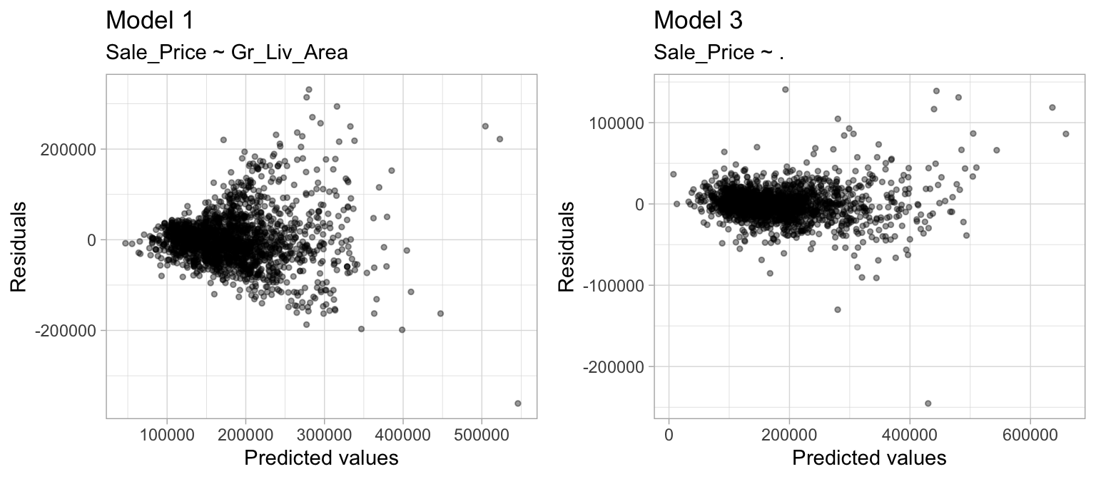

Figure 4.4: Linear regression assumes constant variance among the residuals. model1 (left) shows definitive signs of heteroskedasticity whereas model3 (right) appears to have constant variance.

3. No autocorrelation: Linear regression assumes the errors are independent and uncorrelated. If in fact, there is correlation among the errors, then the estimated standard errors of the coefficients will be biased leading to prediction intervals being narrower than they should be. For example, the left plot in Figure 4.5 displays the residuals (\(y\)-axis) vs. the observation ID (\(x\)-axis) for model1. A clear pattern exists suggesting that information about \(\epsilon_1\) provides information about \(\epsilon_2\).

This pattern is a result of the data being ordered by neighborhood, which we have not accounted for in this model. Consequently, the residuals for homes in the same neighborhood are correlated (homes within a neighborhood are typically the same size and can often contain similar features). Since the Neighborhood predictor is included in model3 (right plot), the correlation in the errors is reduced.

df1 <- mutate(df1, id = row_number())
df2 <- mutate(df2, id = row_number())

p1 <- ggplot(df1, aes(id, .resid)) + 
  geom_point(size = 1, alpha = .4) +
  xlab("Row ID") +
  ylab("Residuals") +
  ggtitle("Model 1", subtitle = "Correlated residuals.")

p2 <- ggplot(df2, aes(id, .resid)) + 
  geom_point(size = 1, alpha = .4) +
  xlab("Row ID") +
  ylab("Residuals") +
  ggtitle("Model 3", subtitle = "Uncorrelated residuals.")

gridExtra::grid.arrange(p1, p2, nrow = 1)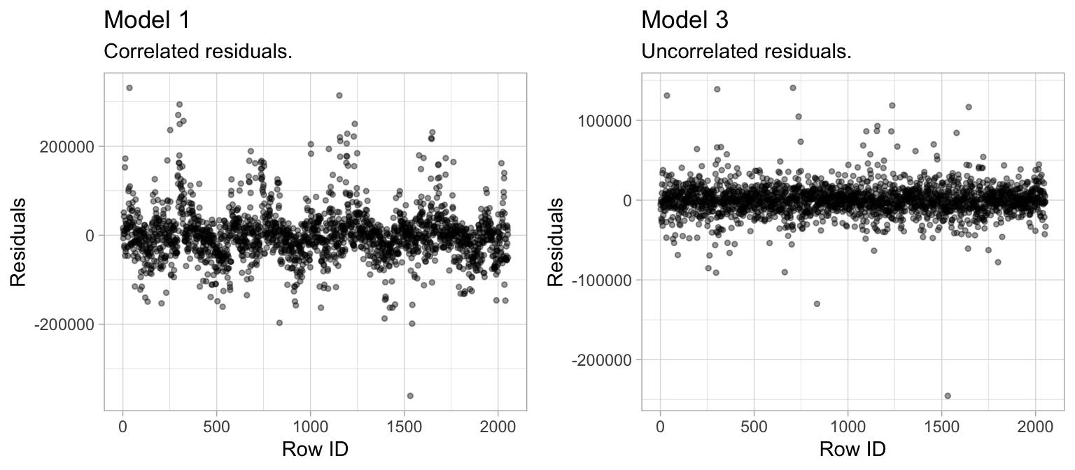

Figure 4.5: Linear regression assumes uncorrelated errors. The residuals in model1 (left) have a distinct pattern suggesting that information about \(\epsilon_1\) provides information about \(\epsilon_2\). Whereas model3 has no signs of autocorrelation.

4. More observations than predictors: Although not an issue with the Ames housing data, when the number of features exceeds the number of observations (\(p > n\)), the OLS estimates are not obtainable. To resolve this issue an analyst can remove variables one-at-a-time until \(p < n\). Although pre-processing tools can be used to guide this manual approach (Kuhn and Johnson 2013, 26:43–47), it can be cumbersome and prone to errors. In Chapter 6 we’ll introduce regularized regression which provides an alternative to OLS that can be used when \(p > n\).

5. No or little multicollinearity: Collinearity refers to the situation in which two or more predictor variables are closely related to one another. The presence of collinearity can pose problems in the OLS, since it can be difficult to separate out the individual effects of collinear variables on the response. In fact, collinearity can cause predictor variables to appear as statistically insignificant when in fact they are significant. This obviously leads to an inaccurate interpretation of coefficients and makes it difficult to identify influential predictors.

In ames, for example, Garage_Area and Garage_Cars are two variables that have a correlation of 0.89 and both variables are strongly related to our response variable (Sale_Price). Looking at our full model where both of these variables are included, we see that Garage_Cars is found to be statistically significant but Garage_Area is not:

# fit with two strongly correlated variables
summary(cv_model3) %>%
  broom::tidy() %>%
  filter(term %in% c("Garage_Area", "Garage_Cars"))
## # A tibble: 2 x 5
##   term        estimate std.error statistic p.value
##   <chr>          <dbl>     <dbl>     <dbl>   <dbl>
## 1 Garage_Cars   3021.    1771.        1.71 0.0882 
## 2 Garage_Area     19.7      6.03      3.26 0.00112

However, if we refit the full model without Garage_Cars, the coefficient estimate for Garage_Area increases two fold and becomes statistically significant.

# model without Garage_Area
set.seed(123)
mod_wo_Garage_Cars <- train(
  Sale_Price ~ ., 
  data = select(ames_train, -Garage_Cars), 
  method = "lm",
  trControl = trainControl(method = "cv", number = 10)
)

summary(mod_wo_Garage_Cars) %>%
  broom::tidy() %>%
  filter(term == "Garage_Area")
## # A tibble: 1 x 5
##   term        estimate std.error statistic  p.value
##   <chr>          <dbl>     <dbl>     <dbl>    <dbl>
## 1 Garage_Area     27.0      4.21      6.43 1.69e-10

This reflects the instability in the linear regression model caused by between-predictor relationships; this instability also gets propagated directly to the model predictions. Considering 16 of our 34 numeric predictors have a medium to strong correlation (Chapter 17), the biased coefficients of these predictors are likely restricting the predictive accuracy of our model. How can we control for this problem? One option is to manually remove the offending predictors (one-at-a-time) until all pairwise correlations are below some pre-determined threshold. However, when the number of predictors is large such as in our case, this becomes tedious. Moreover, multicollinearity can arise when one feature is linearly related to two or more features (which is more difficult to detect²⁰). In these cases, manual removal of specific predictors may not be possible. Consequently, the following sections offers two simple extensions of linear regression where dimension reduction is applied prior to performing linear regression. Chapter 6 offers a modified regression approach that helps to deal with the problem. And future chapters provide alternative methods that are less affected by multicollinearity.

4.6 Principal component regression

As mentioned in Section 3.7 and fully discussed in Chapter 17, principal components analysis can be used to represent correlated variables with a smaller number of uncorrelated features (called principle components) and the resulting components can be used as predictors in a linear regression model. This two-step process is known as principal component regression (PCR) (Massy 1965) and is illustrated in Figure 4.6.

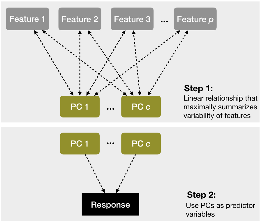
Figure 4.6: A depiction of the steps involved in performing principal component regression.

Performing PCR with caret is an easy extension from our previous model. We simply specify method = "pcr" within train() to perform PCA on all our numeric predictors prior to fitting the model. Often, we can greatly improve performance by only using a small subset of all principal components as predictors. Consequently, you can think of the number of principal components as a tuning parameter (see Section 2.5.3). The following performs cross-validated PCR with \(1, 2, \dots, 100\) principal components, and Figure 4.7 illustrates the cross-validated RMSE. You can see a significant drop in prediction error from our previous linear models using just five principal components followed by a gradual decrease thereafter. However, you may realize that it takes nearly 100 principal components to reach a minimum RMSE (see cv_model_pcr for a comparison of the cross-validated results).

Note in the below example we use preProcess to remove near-zero variance features and center/scale the numeric features. We then use method = “pcr”. This is equivalent to creating a blueprint as illustrated in Section 3.8.3 to remove near-zero variance features, center/scale the numeric features, perform PCA on the numeric features, then feeding that blueprint into train() with method = “lm”.

# perform 10-fold cross validation on a PCR model tuning the 
# number of principal components to use as predictors from 1-100
set.seed(123)
cv_model_pcr <- train(
  Sale_Price ~ ., 
  data = ames_train, 
  method = "pcr",
  trControl = trainControl(method = "cv", number = 10),
  preProcess = c("zv", "center", "scale"),
  tuneLength = 100
  )

# model with lowest RMSE
cv_model_pcr$bestTune
##    ncomp
## 97    97

# results for model with lowest RMSE
cv_model_pcr$results %>%
  dplyr::filter(ncomp == pull(cv_model_pcr$bestTune))
##   ncomp     RMSE  Rsquared      MAE   RMSESD RsquaredSD    MAESD
## 1    97 30135.51 0.8615453 20143.42 5191.887 0.03764501 1696.534

# plot cross-validated RMSE
ggplot(cv_model_pcr)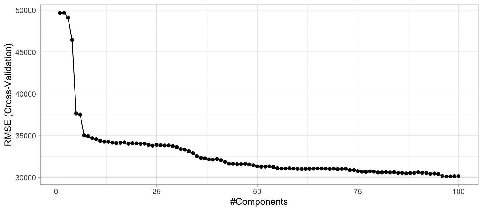

Figure 4.7: The 10-fold cross validation RMSE obtained using PCR with 1-100 principal components.

By controlling for multicollinearity with PCR, we can experience significant improvement in our predictive accuracy compared to the previously obtained linear models (reducing the cross-validated RMSE from about $37,000 to nearly $30,000), which beats the k-nearest neighbor model illustrated in Section 3.8.3. It’s important to note that since PCR is a two step process, the PCA step does not consider any aspects of the response when it selects the components. Consequently, the new predictors produced by the PCA step are not designed to maximize the relationship with the response. Instead, it simply seeks to reduce the variability present throughout the predictor space. If that variability happens to be related to the response variability, then PCR has a good chance to identify a predictive relationship, as in our case. If, however, the variability in the predictor space is not related to the variability of the response, then PCR can have difficulty identifying a predictive relationship when one might actually exists (i.e., we may actually experience a decrease in our predictive accuracy). An alternative approach to reduce the impact of multicollinearity is partial least squares.

4.7 Partial least squares

Partial least squares (PLS) can be viewed as a supervised dimension reduction procedure (Kuhn and Johnson 2013). Similar to PCR, this technique also constructs a set of linear combinations of the inputs for regression, but unlike PCR it uses the response variable to aid the construction of the principal components as illustrated in Figure 4.8²¹. Thus, we can think of PLS as a supervised dimension reduction procedure that finds new features that not only captures most of the information in the original features, but also are related to the response.

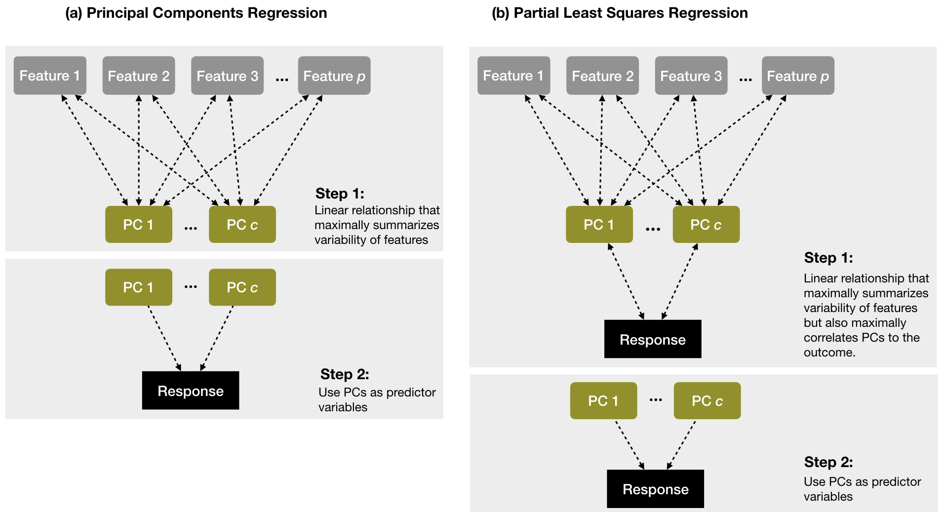
Figure 4.8: A diagram depicting the differences between PCR (left) and PLS (right). PCR finds principal components (PCs) that maximally summarize the features independent of the response variable and then uses those PCs as predictor variables. PLS finds components that simultaneously summarize variation of the predictors while being optimally correlated with the outcome and then uses those PCs as predictors.

We illustrate PLS with some exemplar data²². Figure 4.9 illustrates that the first two PCs when using PCR have very little relationship to the response variable; however, the first two PCs when using PLS have a much stronger association to the response.

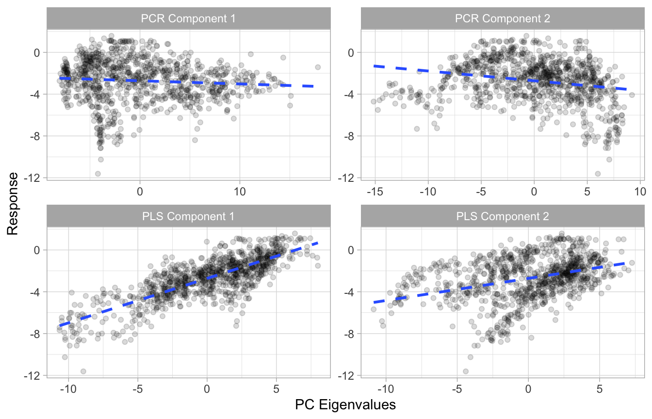
Figure 4.9: Illustration showing that the first two PCs when using PCR have very little relationship to the response variable (top row); however, the first two PCs when using PLS have a much stronger association to the response (bottom row).

Referring to Equation (17.1) in Chapter 17, PLS will compute the first principal (\(z_1\)) by setting each \(\phi_{j1}\) to the coefficient from a SLR model of \(y\) onto that respective \(x_j\). One can show that this coefficient is proportional to the correlation between \(y\) and \(x_j\). Hence, in computing \(z_1 = \sum^p_{j=1} \phi_{j1}x_j\), PLS places the highest weight on the variables that are most strongly related to the response.

To compute the second PC (\(z_2\)), we first regress each variable on \(z_1\). The residuals from this regression capture the remaining signal that has not been explained by the first PC. We substitute these residual values for the predictor values in Equation (17.2) in Chapter 17. This process continues until all \(m\) components have been computed and then we use OLS to regress the response on \(z_1, \dots, z_m\).

See J. Friedman, Hastie, and Tibshirani (2001) and Geladi and Kowalski (1986) for a thorough discussion of PLS.

Similar to PCR, we can easily fit a PLS model by changing the method argument in train(). As with PCR, the number of principal components to use is a tuning parameter that is determined by the model that maximizes predictive accuracy (minimizes RMSE in this case). The following performs cross-validated PLS with \(1, 2, \dots, 30\) PCs, and Figure 4.10 shows the cross-validated RMSEs. You can see a greater drop in prediction error compared to PCR and we reach this minimum RMSE with far less principal components because they are guided by the response.

# perform 10-fold cross validation on a PLS model tuning the 
# number of principal components to use as predictors from 1-30
set.seed(123)
cv_model_pls <- train(
  Sale_Price ~ ., 
  data = ames_train, 
  method = "pls",
  trControl = trainControl(method = "cv", number = 10),
  preProcess = c("zv", "center", "scale"),
  tuneLength = 30
)

# model with lowest RMSE
cv_model_pls$bestTune
##    ncomp
## 20    20

# results for model with lowest RMSE
cv_model_pls$results %>%
  dplyr::filter(ncomp == pull(cv_model_pls$bestTune))
##   ncomp     RMSE  Rsquared      MAE   RMSESD RsquaredSD   MAESD
## 1    20 25459.51 0.8998194 16022.68 5243.478 0.04278512 1665.61

# plot cross-validated RMSE
ggplot(cv_model_pls)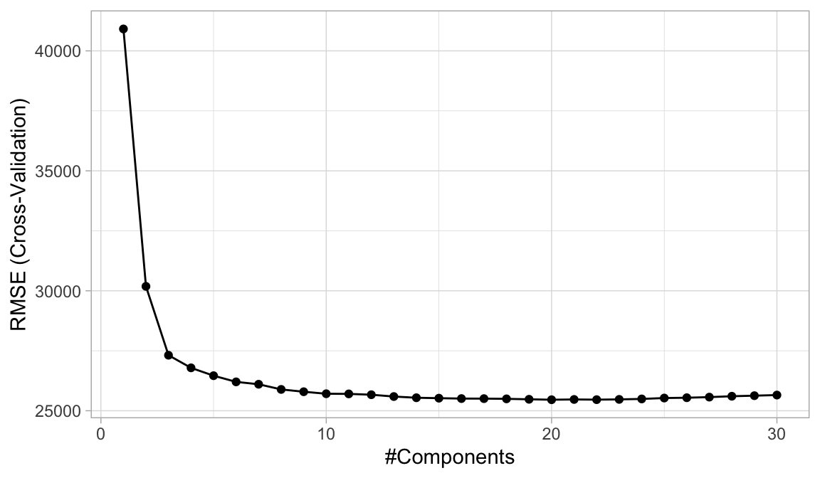

Figure 4.10: The 10-fold cross valdation RMSE obtained using PLS with 1-30 principal components.

4.8 Feature interpretation

Once we’ve found the model that maximizes the predictive accuracy, our next goal is to interpret the model structure. Linear regression models provide a very intuitive model structure as they assume a monotonic linear relationship between the predictor variables and the response. The linear relationship part of that statement just means, for a given predictor variable, it assumes for every one unit change in a given predictor variable there is a constant change in the response. As discussed earlier in the chapter, this constant rate of change is provided by the coefficient for a predictor. The monotonic relationship means that a given predictor variable will always have a positive or negative relationship. But how do we determine the most influential variables?

Variable importance seeks to identify those variables that are most influential in our model. For linear regression models, this is most often measured by the absolute value of the t-statistic for each model parameter used; though simple, the results can be hard to interpret when the model includes interaction effects and complex transformations (in Chapter 16 we’ll discuss model-agnostic approaches that don’t have this issue). For a PLS model, variable importance can be computed using the weighted sums of the absolute regression coefficients. The weights are a function of the reduction of the RSS across the number of PLS components and are computed separately for each outcome. Therefore, the contribution of the coefficients are weighted proportionally to the reduction in the RSS.

We can use vip::vip() to extract and plot the most important variables. The importance measure is normalized from 100 (most important) to 0 (least important). Figure 4.11 illustrates that the top 4 most important variables are Gr_liv_Area, Total_Bsmt_SF, First_Flr_SF, and Garage_Area respectively.

vip(cv_model_pls, num_features = 20, method = "model")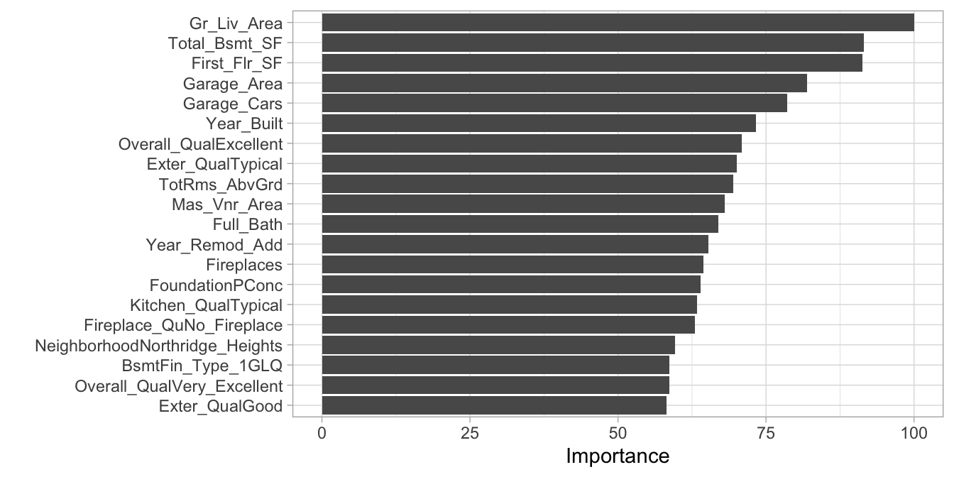

Figure 4.11: Top 20 most important variables for the PLS model.

As stated earlier, linear regression models assume a monotonic linear relationship. To illustrate this, we can construct partial dependence plots (PDPs). PDPs plot the change in the average predicted value (\(\widehat{y}\)) as specified feature(s) vary over their marginal distribution. As you will see in later chapters, PDPs become more useful when non-linear relationships are present (we discuss PDPs and other ML interpretation techniques in Chapter 16). However, PDPs of linear models help illustrate how a fixed change in \(x_i\) relates to a fixed linear change in \(\widehat{y}_i\) while taking into account the average effect of all the other features in the model (for linear models, the slope of the PDP is equal to the corresponding features of the OLS coefficient).

The pdp package (Brandon Greenwell 2018) provides convenient functions for computing and plotting PDPs. For example, the following code chunk would plot the PDP for the Gr_Liv_Area predictor.

pdp::partial(cv_model_pls, "Gr_Liv_Area", grid.resolution = 20, plot = TRUE)

All four of the most important predictors have a positive relationship with sale price; however, we see that the slope (\(\widehat{\beta}_i\)) is steepest for the most important predictor and gradually decreases for less important variables.

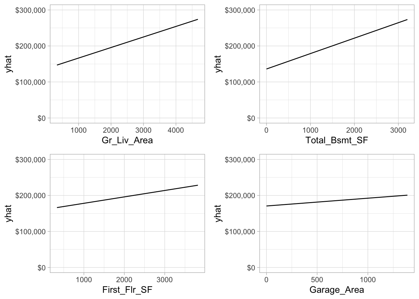
Figure 4.12: Partial dependence plots for the first four most important variables.

4.9 Final thoughts

Linear regression is usually the first supervised learning algorithm you will learn. The approach provides a solid fundamental understanding of the supervised learning task; however, as we’ve discussed there are several concerns that result from the assumptions required. Although extensions of linear regression that integrate dimension reduction steps into the algorithm can help address some of the problems with linear regression, more advanced supervised algorithms typically provide greater flexibility and improved accuracy. Nonetheless, understanding linear regression provides a foundation that will serve you well in learning these more advanced methods.

References

Faraway, Julian J. 2016b. Linear Models with R. Chapman; Hall/CRC.

Friedman, Jerome, Trevor Hastie, and Robert Tibshirani. 2001. The Elements of Statistical Learning. Vol. 1. Springer Series in Statistics New York, NY, USA:

Geladi, Paul, and Bruce R Kowalski. 1986. “Partial Least-Squares Regression: A Tutorial.” Analytica Chimica Acta 185. Elsevier: 1–17.

Greenwell, Brandon. 2018. Pdp: Partial Dependence Plots. https://CRAN.R-project.org/package=pdp.

Kuhn, Max, and Kjell Johnson. 2013. Applied Predictive Modeling. Vol. 26. Springer.

Kutner, M. H., C. J. Nachtsheim, J. Neter, and W. Li. 2005. Applied Linear Statistical Models. 5th ed. McGraw Hill.

Massy, William F. 1965. “Principal Components Regression in Exploratory Statistical Research.” Journal of the American Statistical Association 60 (309). Taylor & Francis Group: 234–56.

---

18. Transformations of the features serve a number of purposes (e.g., modeling nonlinear relationships or alleviating departures from common regression assumptions). See Kutner et al. (2005) for details.↩

19. Although general cross-validation is not available in lm() alone, a simple metric called the PRESS statistic, for PREdictive Sum of Square, (equivalent to a leave-one-out cross-validated RMSE) can be computed by summing the PRESS residuals which are available using rstandard(<lm-model-name>, type = "predictive"). See ?rstandard for details.↩

20. In such cases we can use a statistic called the variance inflation factor which tries to capture how strongly each feature is linearly related to all the others predictors in a model.↩

21. Figure 4.8 was inspired by, and modified from, Chapter 6 in Kuhn and Johnson (2013).↩

22. This is actually using the solubility data that is provided by the AppliedPredictiveModeling package (Kuhn and Johnson 2018).↩