Chapter 3 Feature & Target Engineering

Data preprocessing and engineering techniques generally refer to the addition, deletion, or transformation of data. The time spent on identifying data engineering needs can be significant and requires you to spend substantial time understanding your data…or as Leo Breiman said “live with your data before you plunge into modeling” (Breiman and others 2001, 201). Although this book primarily focuses on applying machine learning algorithms, feature engineering can make or break an algorithm’s predictive ability and deserves your continued focus and education.

We will not cover all the potential ways of implementing feature engineering; however, we’ll cover several fundamental preprocessing tasks that can potentially significantly improve modeling performance. Moreover, different models have different sensitivities to the type of target and feature values in the model and we will try to highlight some of these concerns. For more in depth coverage of feature engineering, please refer to Kuhn and Johnson (2019) and Zheng and Casari (2018).

3.1 Prerequisites

This chapter leverages the following packages:

# Helper packages
library(dplyr)    # for data manipulation
library(ggplot2)  # for awesome graphics
library(visdat)   # for additional visualizations

# Feature engineering packages
library(caret)    # for various ML tasks
library(recipes)  # for feature engineering tasks

We’ll also continue working with the ames_train data set created in Section 2.7:

3.2 Target engineering

Although not always a requirement, transforming the response variable can lead to predictive improvement, especially with parametric models (which require that certain assumptions about the model be met). For instance, ordinary linear regression models assume that the prediction errors (and hence the response) are normally distributed. This is usually fine, except when the prediction target has heavy tails (i.e., outliers) or is skewed in one direction or the other. In these cases, the normality assumption likely does not hold. For example, as we saw in the data splitting section (2.2), the response variable for the Ames housing data (Sale_Price) is right (or positively) skewed as illustrated in Figure 3.1 (ranging from $12,789 to $755,000). A simple linear model, say $\text{Sale_Price}=\beta_{0} + \beta_{1} \text{Year_Built} + \epsilon$, often assumes the error term $\epsilon$ (and hence Sale_Price) is normally distributed; fortunately, a simple log (or similar) transformation of the response can often help alleviate this concern as Figure 3.1 illustrates.

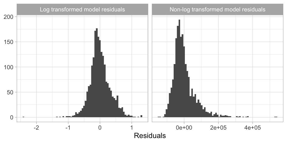
Figure 3.1: Transforming the response variable to minimize skewness can resolve concerns with non-normally distributed errors.

Furthermore, using a log (or other) transformation to minimize the response skewness can be used for shaping the business problem as well. For example, in the House Prices: Advanced Regression Techniques Kaggle competition¹¹, which used the Ames housing data, the competition focused on using a log transformed Sale Price response because “…taking logs means that errors in predicting expensive houses and cheap houses will affect the result equally.” This would be an alternative to using the root mean squared logarithmic error (RMSLE) loss function as discussed in Section 2.6.

There are two main approaches to help correct for positively skewed target variables:

Option 1: normalize with a log transformation. This will transform most right skewed distributions to be approximately normal. One way to do this is to simply log transform the training and test set in a manual, single step manner similar to:

transformed_response <- log(ames_train$Sale_Price)

However, we should think of the preprocessing as creating a blueprint to be re-applied strategically. For this, you can use the recipe package or something similar (e.g., caret::preProcess()). This will not return the actual log transformed values but, rather, a blueprint to be applied later.

# log transformation
ames_recipe <- recipe(Sale_Price ~ ., data = ames_train) %>%
  step_log(all_outcomes())

ames_recipe
## Data Recipe
## 
## Inputs:
## 
##       role #variables
##    outcome          1
##  predictor         80
## 
## Operations:
## 
## Log transformation on all_outcomes

If your response has negative values or zeros then a log transformation will produce NaNs and -Infs, respectively (you cannot take the logarithm of a negative number). If the nonpositive response values are small (say between -0.99 and 0) then you can apply a small offset such as in log1p() which adds 1 to the value prior to applying a log transformation (you can do the same within step_log() by using the offset argument). If your data consists of values $\le -1$, use the Yeo-Johnson transformation mentioned next.

log(-0.5)
## [1] NaN
log1p(-0.5)
## [1] -0.6931472

Option 2: use a Box Cox transformation. A Box Cox transformation is more flexible than (but also includes as a special case) the log transformation and will find an appropriate transformation from a family of power transforms that will transform the variable as close as possible to a normal distribution (Box and Cox 1964; Carroll and Ruppert 1981). At the core of the Box Cox transformation is an exponent, lambda ($\lambda$), which varies from -5 to 5. All values of $\lambda$ are considered and the optimal value for the given data is estimated from the training data; The “optimal value” is the one which results in the best transformation to an approximate normal distribution. The transformation of the response $Y$ has the form:

\[ \begin{equation} y(\lambda) = \begin{cases} \frac{Y^\lambda-1}{\lambda}, & \text{if}\ \lambda \neq 0 \\ \log\left(Y\right), & \text{if}\ \lambda = 0. \end{cases} \end{equation} \]

Be sure to compute the lambda on the training set and apply that same lambda to both the training and test set to minimize data leakage. The recipes package automates this process for you.

If your response has negative values, the Yeo-Johnson transformation is very similar to the Box-Cox but does not require the input variables to be strictly positive. To apply, use step_YeoJohnson().

Figure 3.2 illustrates that the log transformation and Box Cox transformation both do about equally well in transforming Sale_Price to look more normally distributed.

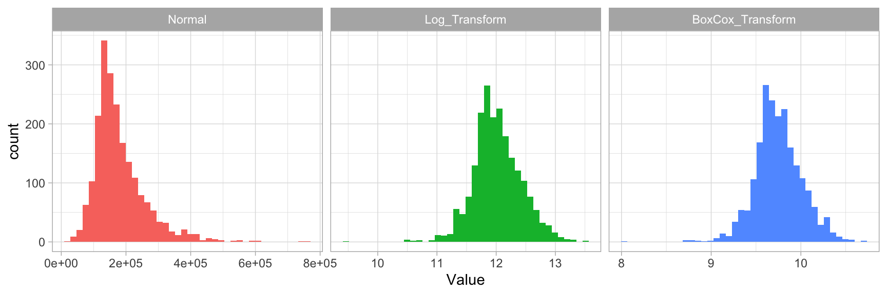
Figure 3.2: Response variable transformations.

Note that when you model with a transformed response variable, your predictions will also be on the transformed scale. You will likely want to undo (or re-transform) your predicted values back to their normal scale so that decision-makers can more easily interpret the results. This is illustrated in the following code chunk:

# Log transform a value
y <- log(10)

# Undo log-transformation
exp(y)
## [1] 10

# Box Cox transform a value
y <- forecast::BoxCox(10, lambda)

# Inverse Box Cox function
inv_box_cox <- function(x, lambda) {
  # for Box-Cox, lambda = 0 --> log transform
  if (lambda == 0) exp(x) else (lambda*x + 1)^(1/lambda) 
}

# Undo Box Cox-transformation
inv_box_cox(y, lambda)
## [1] 10
## attr(,"lambda")
## [1] -0.03616899

3.3 Dealing with missingness

Data quality is an important issue for any project involving analyzing data. Data quality issues deserve an entire book in their own right, and a good reference is The Quartz guide to bad data.¹² One of the most common data quality concerns you will run into is missing values.

Data can be missing for many different reasons; however, these reasons are usually lumped into two categories: informative missingness (Kuhn and Johnson 2013) and missingness at random (Little and Rubin 2014). Informative missingness implies a structural cause for the missing value that can provide insight in its own right; whether this be deficiencies in how the data was collected or abnormalities in the observational environment. Missingness at random implies that missing values occur independent of the data collection process¹³.

The category that drives missing values will determine how you handle them. For example, we may give values that are driven by informative missingness their own category (e.g., "None") as their unique value may affect predictive performance. Whereas values that are missing at random may deserve deletion¹⁴ or imputation.

Furthermore, different machine learning models handle missingness differently. Most algorithms cannot handle missingness (e.g., generalized linear models and their cousins, neural networks, and support vector machines) and, therefore, require them to be dealt with beforehand. A few models (mainly tree-based), have built-in procedures to deal with missing values. However, since the modeling process involves comparing and contrasting multiple models to identify the optimal one, you will want to handle missing values prior to applying any models so that your algorithms are based on the same data quality assumptions.

3.3.1 Visualizing missing values

It is important to understand the distribution of missing values (i.e., NA) in any data set. So far, we have been using a pre-processed version of the Ames housing data set (via the AmesHousing::make_ames() function). However, if we use the raw Ames housing data (via AmesHousing::ames_raw), there are actually 13,997 missing values—there is at least one missing values in each row of the original data!

sum(is.na(AmesHousing::ames_raw))
## [1] 13997

It is important to understand the distribution of missing values in a data set in order to determine the best approach for preprocessing. Heat maps are an efficient way to visualize the distribution of missing values for small- to medium-sized data sets. The code is.na(<data-frame-name>) will return a matrix of the same dimension as the given data frame, but each cell will contain either TRUE (if the corresponding value is missing) or FALSE (if the corresponding value is not missing). To construct such a plot, we can use R’s built-in heatmap() or image() functions, or ggplot2’s geom_raster() function, among others; Figure 3.3 illustrates geom_raster(). This allows us to easily see where the majority of missing values occur (i.e., in the variables Alley, Fireplace Qual, Pool QC, Fence, and Misc Feature). Due to their high frequency of missingness, these variables would likely need to be removed prior to statistical analysis, or imputed. We can also spot obvious patterns of missingness. For example, missing values appear to occur within the same observations across all garage variables.

AmesHousing::ames_raw %>%
  is.na() %>%
  reshape2::melt() %>%
  ggplot(aes(Var2, Var1, fill=value)) + 
    geom_raster() + 
    coord_flip() +
    scale_y_continuous(NULL, expand = c(0, 0)) +
    scale_fill_grey(name = "", 
                    labels = c("Present", 
                               "Missing")) +
    xlab("Observation") +
    theme(axis.text.y  = element_text(size = 4))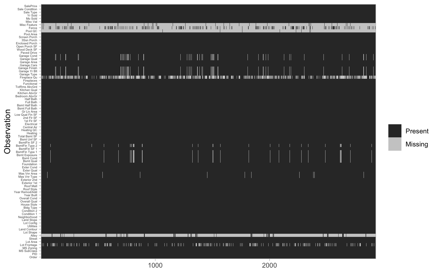

Figure 3.3: Heat map of missing values in the raw Ames housing data.

Digging a little deeper into these variables, we might notice that Garage_Cars and Garage_Area contain the value 0 whenever the other Garage_xx variables have missing values (i.e. a value of NA). This might be because they did not have a way to identify houses with no garages when the data were originally collected, and therefore, all houses with no garage were identified by including nothing. Since this missingness is informative, it would be appropriate to impute NA with a new category level (e.g., "None") for these garage variables. Circumstances like this tend to only become apparent upon careful descriptive and visual examination of the data!

AmesHousing::ames_raw %>% 
  filter(is.na(`Garage Type`)) %>% 
  select(`Garage Type`, `Garage Cars`, `Garage Area`)
## # A tibble: 157 x 3
##    `Garage Type` `Garage Cars` `Garage Area`
##    <chr>                 <int>         <int>
##  1 <NA>                      0             0
##  2 <NA>                      0             0
##  3 <NA>                      0             0
##  4 <NA>                      0             0
##  5 <NA>                      0             0
##  6 <NA>                      0             0
##  7 <NA>                      0             0
##  8 <NA>                      0             0
##  9 <NA>                      0             0
## 10 <NA>                      0             0
## # … with 147 more rows

The vis_miss() function in R package visdat (Tierney 2019) also allows for easy visualization of missing data patterns (with sorting and clustering options). We illustrate this functionality below using the raw Ames housing data (Figure 3.4). The columns of the heat map represent the 82 variables of the raw data and the rows represent the observations. Missing values (i.e., NA) are indicated via a black cell. The variables and NA patterns have been clustered by rows (i.e., cluster = TRUE).

vis_miss(AmesHousing::ames_raw, cluster = TRUE)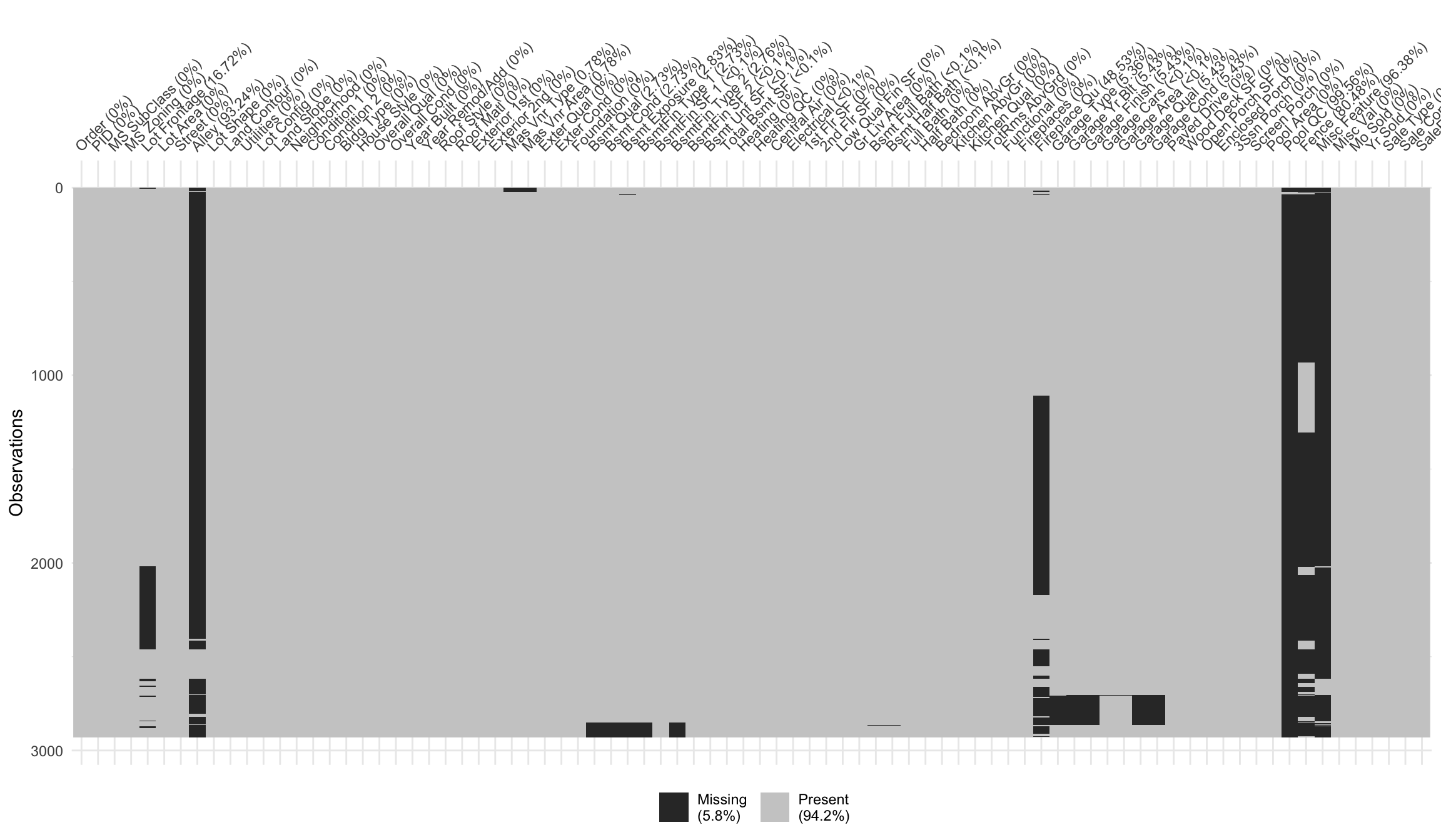

Figure 3.4: Visualizing missing data patterns in the raw Ames housing data.

Data can be missing for different reasons. Perhaps the values were never recorded (or lost in translation), or it was recorded in error (a common feature of data entered by hand). Regardless, it is important to identify and attempt to understand how missing values are distributed across a data set as it can provide insight into how to deal with these observations.

3.3.2 Imputation

Imputation is the process of replacing a missing value with a substituted, “best guess” value. Imputation should be one of the first feature engineering steps you take as it will affect any downstream preprocessing¹⁵.

3.3.2.1 Estimated statistic

An elementary approach to imputing missing values for a feature is to compute descriptive statistics such as the mean, median, or mode (for categorical) and use that value to replace NAs. Although computationally efficient, this approach does not consider any other attributes for a given observation when imputing (e.g., a female patient that is 63 inches tall may have her weight imputed as 175 lbs since that is the average weight across all observations which contains 65% males that average a height of 70 inches).

An alternative is to use grouped statistics to capture expected values for observations that fall into similar groups. However, this becomes infeasible for larger data sets. Modeling imputation can automate this process for you and the two most common methods include K-nearest neighbor and tree-based imputation, which are discussed next.

However, it is important to remember that imputation should be performed within the resampling process and as your data set gets larger, repeated model-based imputation can compound the computational demands. Thus, you must weigh the pros and cons of the two approaches. The following would build onto our ames_recipe and impute all missing values for the Gr_Liv_Area variable with the median value:

ames_recipe %>%
  step_medianimpute(Gr_Liv_Area)
## Data Recipe
## 
## Inputs:
## 
##       role #variables
##    outcome          1
##  predictor         80
## 
## Operations:
## 
## Log transformation on all_outcomes
## Median Imputation for Gr_Liv_Area

Use step_modeimpute() to impute categorical features with the most common value.

3.3.2.2 K-nearest neighbor

K-nearest neighbor (KNN) imputes values by identifying observations with missing values, then identifying other observations that are most similar based on the other available features, and using the values from these nearest neighbor observations to impute missing values.

We discuss KNN for predictive modeling in Chapter 8; the imputation application works in a similar manner. In KNN imputation, the missing value for a given observation is treated as the targeted response and is predicted based on the average (for quantitative values) or the mode (for qualitative values) of the k nearest neighbors.

As discussed in Chapter 8, if all features are quantitative then standard Euclidean distance is commonly used as the distance metric to identify the k neighbors and when there is a mixture of quantitative and qualitative features then Gower’s distance (Gower 1971) can be used. KNN imputation is best used on small to moderate sized data sets as it becomes computationally burdensome with larger data sets (Kuhn and Johnson 2019).

As we saw in Section 2.7, k is a tunable hyperparameter. Suggested values for imputation are 5–10 (Kuhn and Johnson 2019). By default, step_knnimpute() will use 5 but can be adjusted with the neighbors argument.

ames_recipe %>%
  step_knnimpute(all_predictors(), neighbors = 6)
## Data Recipe
## 
## Inputs:
## 
##       role #variables
##    outcome          1
##  predictor         80
## 
## Operations:
## 
## Log transformation on all_outcomes
## K-nearest neighbor imputation for all_predictors

3.3.2.3 Tree-based

As previously discussed, several implementations of decision trees (Chapter 9) and their derivatives can be constructed in the presence of missing values. Thus, they provide a good alternative for imputation. As discussed in Chapters 9-11, single trees have high variance but aggregating across many trees creates a robust, low variance predictor. Random forest imputation procedures have been studied (Shah et al. 2014; Stekhoven 2015); however, they require significant computational demands in a resampling environment (Kuhn and Johnson 2019). Bagged trees (Chapter 10) offer a compromise between predictive accuracy and computational burden.

Similar to KNN imputation, observations with missing values are identified and the feature containing the missing value is treated as the target and predicted using bagged decision trees.

ames_recipe %>%
  step_bagimpute(all_predictors())
## Data Recipe
## 
## Inputs:
## 
##       role #variables
##    outcome          1
##  predictor         80
## 
## Operations:
## 
## Log transformation on all_outcomes
## Bagged tree imputation for all_predictors

Figure 3.5 illustrates the differences between mean, KNN, and tree-based imputation on the raw Ames housing data. It is apparent how descriptive statistic methods (e.g., using the mean and median) are inferior to the KNN and tree-based imputation methods.

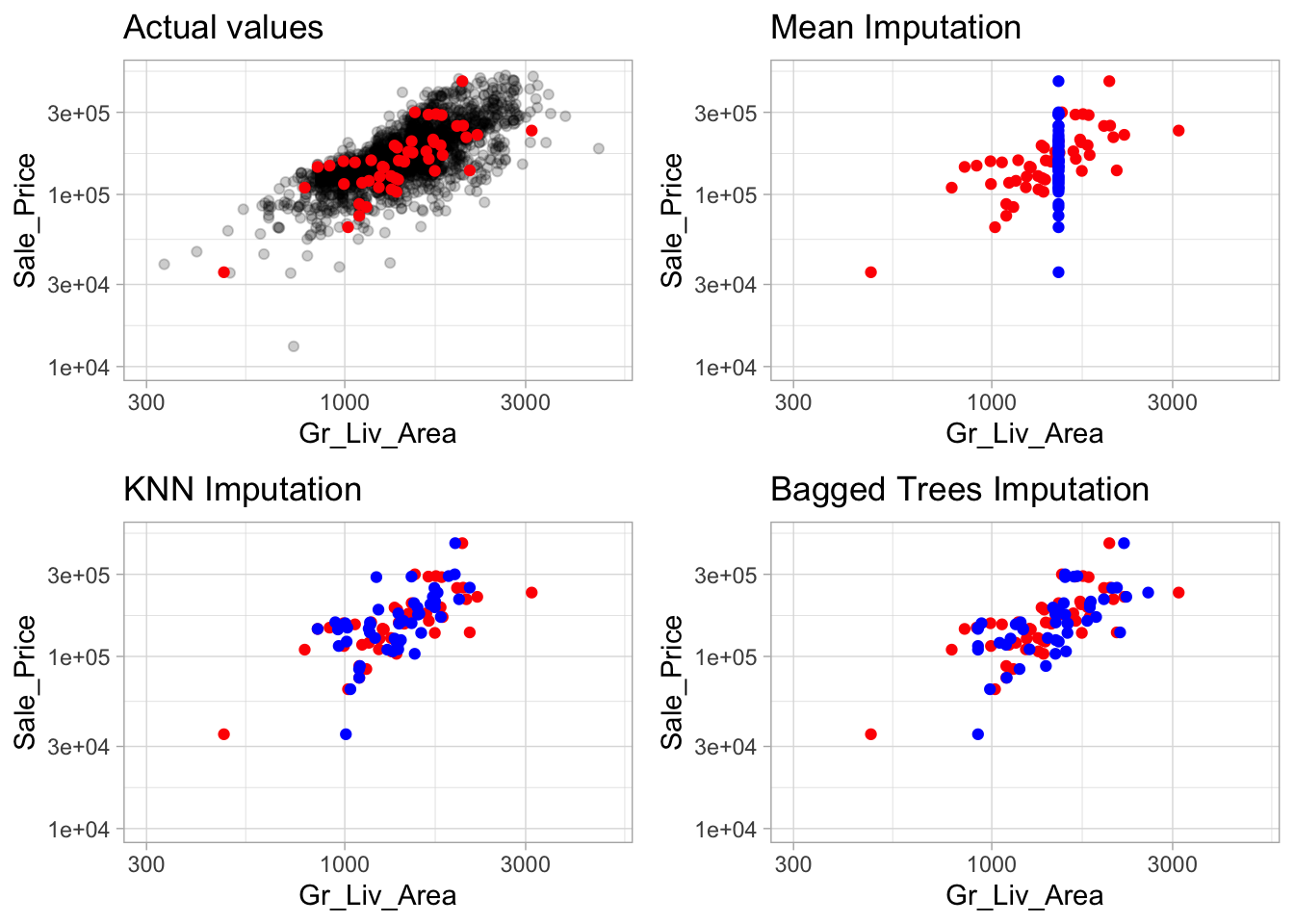
Comparison of three different imputation methods. The red points represent actual values which were removed and made missing and the blue points represent the imputed values. Estimated statistic imputation methods (i.e. mean, median) merely predict the same value for each observation and can reduce the signal between a feature and the response; whereas KNN and tree-based procedures tend to maintain the feature distribution and relationship.

Figure 3.5: Comparison of three different imputation methods. The red points represent actual values which were removed and made missing and the blue points represent the imputed values. Estimated statistic imputation methods (i.e. mean, median) merely predict the same value for each observation and can reduce the signal between a feature and the response; whereas KNN and tree-based procedures tend to maintain the feature distribution and relationship.

3.4 Feature filtering

In many data analyses and modeling projects we end up with hundreds or even thousands of collected features. From a practical perspective, a model with more features often becomes harder to interpret and is costly to compute. Some models are more resistant to non-informative predictors (e.g., the Lasso and tree-based methods) than others as illustrated in Figure 3.6.¹⁶

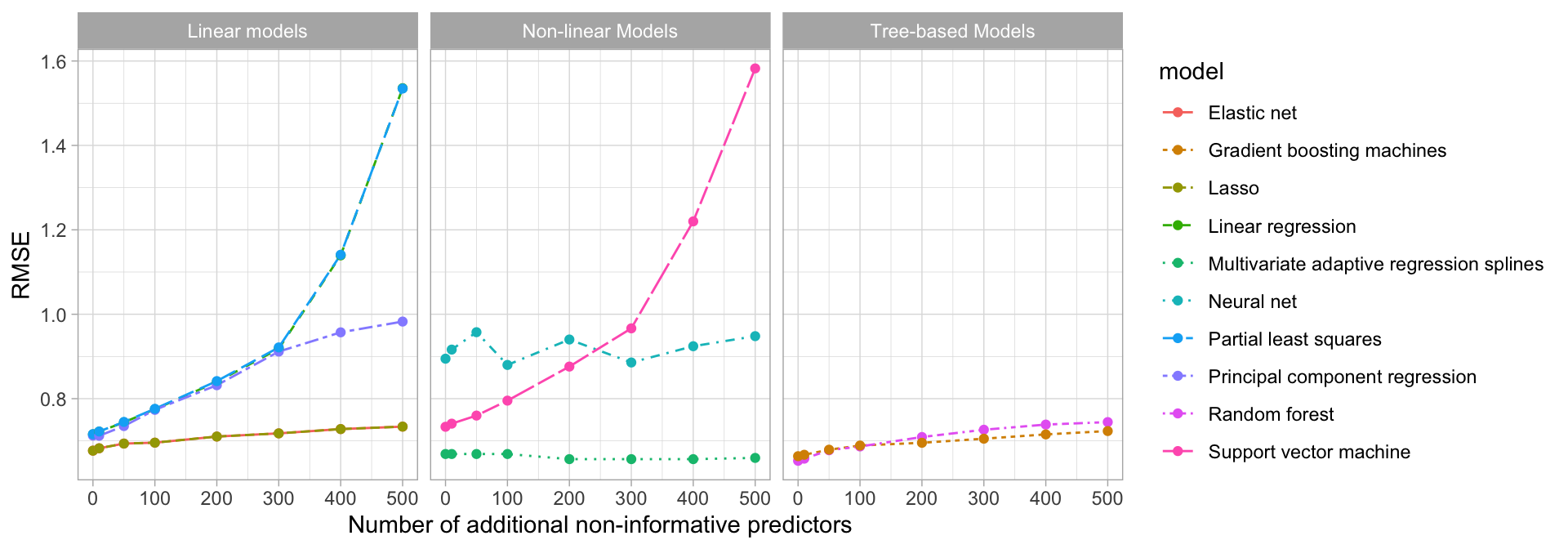
Figure 3.6: Test set RMSE profiles when non-informative predictors are added.

Although the performance of some of our models are not significantly affected by non-informative predictors, the time to train these models can be negatively impacted as more features are added. Figure 3.7 shows the increase in time to perform 10-fold CV on the exemplar data, which consists of 10,000 observations. We see that many algorithms (e.g., elastic nets, random forests, and gradient boosting machines) become extremely time intensive the more predictors we add. Consequently, filtering or reducing features prior to modeling may significantly speed up training time.

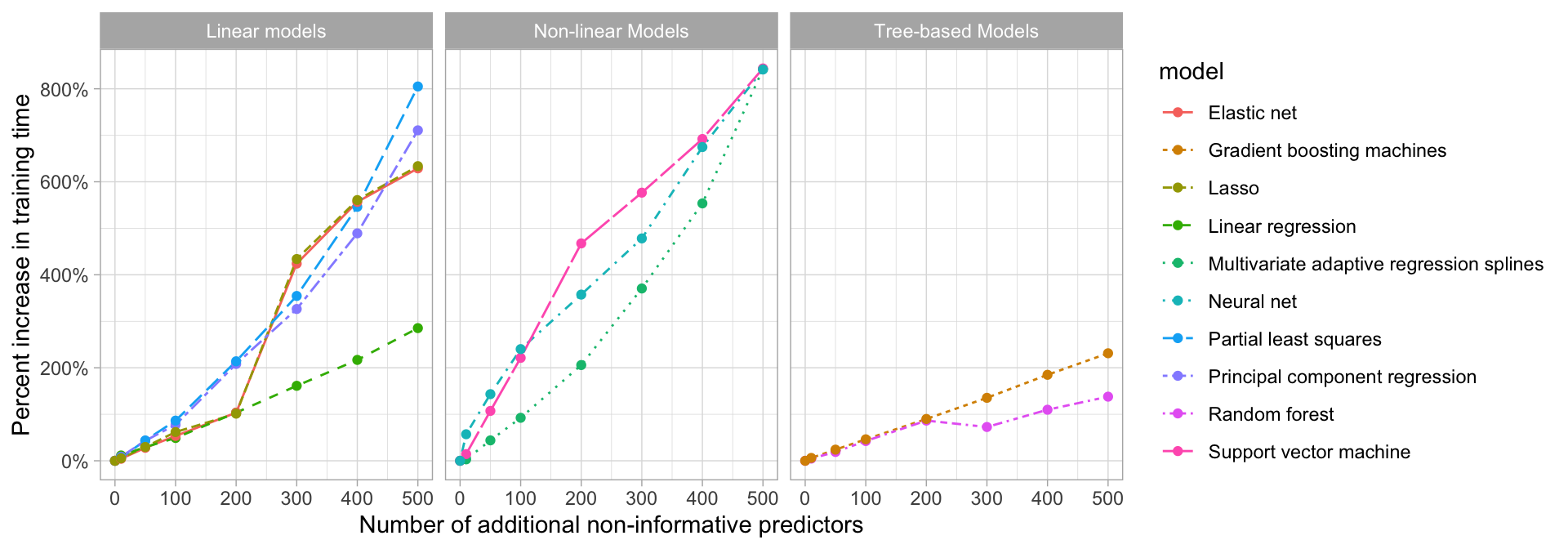
Figure 3.7: Impact in model training time as non-informative predictors are added.

Zero and near-zero variance variables are low-hanging fruit to eliminate. Zero variance variables, meaning the feature only contains a single unique value, provides no useful information to a model. Some algorithms are unaffected by zero variance features. However, features that have near-zero variance also offer very little, if any, information to a model. Furthermore, they can cause problems during resampling as there is a high probability that a given sample will only contain a single unique value (the dominant value) for that feature. A rule of thumb for detecting near-zero variance features is:

The fraction of unique values over the sample size is low (say $\leq 10$%).
The ratio of the frequency of the most prevalent value to the frequency of the second most prevalent value is large (say $\geq 20$%).

If both of these criteria are true then it is often advantageous to remove the variable from the model. For the Ames data, we do not have any zero variance predictors but there are 20 features that meet the near-zero threshold.

caret::nearZeroVar(ames_train, saveMetrics = TRUE) %>% 
  tibble::rownames_to_column() %>% 
  filter(nzv)
##               rowname  freqRatio percentUnique zeroVar  nzv
## 1              Street  292.28571    0.09741841   FALSE TRUE
## 2               Alley   21.76136    0.14612762   FALSE TRUE
## 3        Land_Contour   21.78824    0.19483682   FALSE TRUE
## 4           Utilities 1025.00000    0.14612762   FALSE TRUE
## 5          Land_Slope   23.33333    0.14612762   FALSE TRUE
## 6         Condition_2  225.77778    0.34096444   FALSE TRUE
## 7           Roof_Matl  126.50000    0.24354603   FALSE TRUE
## 8           Bsmt_Cond   19.88043    0.29225524   FALSE TRUE
## 9      BsmtFin_Type_2   22.35897    0.34096444   FALSE TRUE
## 10            Heating   96.23810    0.24354603   FALSE TRUE
## 11    Low_Qual_Fin_SF 1012.00000    1.31514856   FALSE TRUE
## 12      Kitchen_AbvGr   23.10588    0.19483682   FALSE TRUE
## 13         Functional   38.95918    0.34096444   FALSE TRUE
## 14     Enclosed_Porch  107.68750    7.25767170   FALSE TRUE
## 15 Three_season_porch  675.00000    1.12031174   FALSE TRUE
## 16       Screen_Porch  234.87500    4.52995616   FALSE TRUE
## 17          Pool_Area 2045.00000    0.43838285   FALSE TRUE
## 18            Pool_QC  681.66667    0.24354603   FALSE TRUE
## 19       Misc_Feature   31.00000    0.19483682   FALSE TRUE
## 20           Misc_Val  152.76923    1.36385777   FALSE TRUE

We can add step_zv() and step_nzv() to our ames_recipe to remove zero or near-zero variance features.

Other feature filtering methods exist; see Saeys, Inza, and Larrañaga (2007) for a thorough review. Furthermore, several wrapper methods exist that evaluate multiple models using procedures that add or remove predictors to find the optimal combination of features that maximizes model performance (see, for example, Kursa, Rudnicki, and others (2010), Granitto et al. (2006), Maldonado and Weber (2009)). However, this topic is beyond the scope of this book.

3.5 Numeric feature engineering

Numeric features can create a host of problems for certain models when their distributions are skewed, contain outliers, or have a wide range in magnitudes. Tree-based models are quite immune to these types of problems in the feature space, but many other models (e.g., GLMs, regularized regression, KNN, support vector machines, neural networks) can be greatly hampered by these issues. Normalizing and standardizing heavily skewed features can help minimize these concerns.

3.5.1 Skewness

Similar to the process discussed to normalize target variables, parametric models that have distributional assumptions (e.g., GLMs, and regularized models) can benefit from minimizing the skewness of numeric features. When normalizing many variables, it’s best to use the Box-Cox (when feature values are strictly positive) or Yeo-Johnson (when feature values are not strictly positive) procedures as these methods will identify if a transformation is required and what the optimal transformation will be.

Non-parametric models are rarely affected by skewed features; however, normalizing features will not have a negative effect on these models’ performance. For example, normalizing features will only shift the optimal split points in tree-based algorithms. Consequently, when in doubt, normalize.

# Normalize all numeric columns
recipe(Sale_Price ~ ., data = ames_train) %>%
  step_YeoJohnson(all_numeric())                 
## Data Recipe
## 
## Inputs:
## 
##       role #variables
##    outcome          1
##  predictor         80
## 
## Operations:
## 
## Yeo-Johnson transformation on all_numeric

3.5.2 Standardization

We must also consider the scale on which the individual features are measured. What are the largest and smallest values across all features and do they span several orders of magnitude? Models that incorporate smooth functions of input features are sensitive to the scale of the inputs. For example, $5X+2$ is a simple linear function of the input X, and the scale of its output depends directly on the scale of the input. Many algorithms use linear functions within their algorithms, some more obvious (e.g., GLMs and regularized regression) than others (e.g., neural networks, support vector machines, and principal components analysis). Other examples include algorithms that use distance measures such as the Euclidean distance (e.g., k nearest neighbor, k-means clustering, and hierarchical clustering).

For these models and modeling components, it is often a good idea to standardize the features. Standardizing features includes centering and scaling so that numeric variables have zero mean and unit variance, which provides a common comparable unit of measure across all the variables.

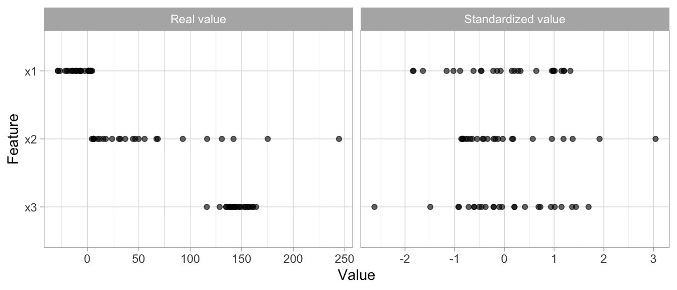
Figure 3.8: Standardizing features allows all features to be compared on a common value scale regardless of their real value differences.

Some packages (e.g., glmnet, and caret) have built-in options to standardize and some do not (e.g., keras for neural networks). However, you should standardize your variables within the recipe blueprint so that both training and test data standardization are based on the same mean and variance. This helps to minimize data leakage.

ames_recipe %>%
  step_center(all_numeric(), -all_outcomes()) %>%
  step_scale(all_numeric(), -all_outcomes())
## Data Recipe
## 
## Inputs:
## 
##       role #variables
##    outcome          1
##  predictor         80
## 
## Operations:
## 
## Log transformation on all_outcomes
## Centering for all_numeric, -, all_outcomes()
## Scaling for all_numeric, -, all_outcomes()

3.6 Categorical feature engineering

Most models require that the predictors take numeric form. There are exceptions; for example, tree-based models naturally handle numeric or categorical features. However, even tree-based models can benefit from preprocessing categorical features. The following sections will discuss a few of the more common approaches to engineer categorical features.

3.6.1 Lumping

Sometimes features will contain levels that have very few observations. For example, there are 28 unique neighborhoods represented in the Ames housing data but several of them only have a few observations.

count(ames_train, Neighborhood) %>% arrange(n)
## # A tibble: 28 x 2
##    Neighborhood                                n
##    <fct>                                   <int>
##  1 Landmark                                    1
##  2 Green_Hills                                 2
##  3 Greens                                      7
##  4 Blueste                                     9
##  5 Northpark_Villa                            17
##  6 Briardale                                  18
##  7 Veenker                                    20
##  8 Bloomington_Heights                        21
##  9 South_and_West_of_Iowa_State_University    30
## 10 Meadow_Village                             30
## # … with 18 more rows

Even numeric features can have similar distributions. For example, Screen_Porch has 92% values recorded as zero (zero square footage meaning no screen porch) and the remaining 8% have unique dispersed values.

count(ames_train, Screen_Porch) %>% arrange(n)
## # A tibble: 93 x 2
##    Screen_Porch     n
##           <int> <int>
##  1           40     1
##  2           80     1
##  3           92     1
##  4           94     1
##  5           99     1
##  6          104     1
##  7          109     1
##  8          110     1
##  9          111     1
## 10          117     1
## # … with 83 more rows

Sometimes we can benefit from collapsing, or “lumping” these into a lesser number of categories. In the above examples, we may want to collapse all levels that are observed in less than 10% of the training sample into an “other” category. We can use step_other() to do so. However, lumping should be used sparingly as there is often a loss in model performance (Kuhn and Johnson 2013).

Tree-based models often perform exceptionally well with high cardinality features and are not as impacted by levels with small representation.

# Lump levels for two features
lumping <- recipe(Sale_Price ~ ., data = ames_train) %>%
  step_other(Neighborhood, threshold = 0.01, 
             other = "other") %>%
  step_other(Screen_Porch, threshold = 0.1, 
             other = ">0")

# Apply this blue print --> you will learn about this at 
# the end of the chapter
apply_2_training <- prep(lumping, training = ames_train) %>%
  bake(ames_train)

# New distribution of Neighborhood
count(apply_2_training, Neighborhood) %>% arrange(n)
## # A tibble: 22 x 2
##    Neighborhood                                n
##    <fct>                                   <int>
##  1 Bloomington_Heights                        21
##  2 South_and_West_of_Iowa_State_University    30
##  3 Meadow_Village                             30
##  4 Clear_Creek                                31
##  5 Stone_Brook                                34
##  6 Northridge                                 48
##  7 Timberland                                 55
##  8 Iowa_DOT_and_Rail_Road                     62
##  9 Crawford                                   72
## 10 Mitchell                                   74
## # … with 12 more rows

# New distribution of Screen_Porch
count(apply_2_training, Screen_Porch) %>% arrange(n)
## # A tibble: 2 x 2
##   Screen_Porch     n
##   <fct>        <int>
## 1 >0             174
## 2 0             1879

3.6.2 One-hot & dummy encoding

Many models require that all predictor variables be numeric. Consequently, we need to intelligently transform any categorical variables into numeric representations so that these algorithms can compute. Some packages automate this process (e.g., h2o and caret) while others do not (e.g., glmnet and keras). There are many ways to recode categorical variables as numeric (e.g., one-hot, ordinal, binary, sum, and Helmert).

The most common is referred to as one-hot encoding, where we transpose our categorical variables so that each level of the feature is represented as a boolean value. For example, one-hot encoding the left data frame in Figure 3.9 results in X being converted into three columns, one for each level. This is called less than full rank encoding . However, this creates perfect collinearity which causes problems with some predictive modeling algorithms (e.g., ordinary linear regression and neural networks). Alternatively, we can create a full-rank encoding by dropping one of the levels (level c has been dropped). This is referred to as dummy encoding.

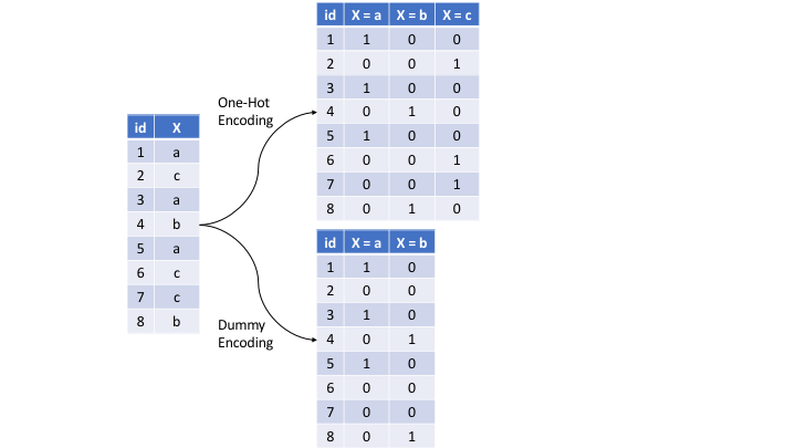
Figure 3.9: Eight observations containing a categorical feature X and the difference in how one-hot and dummy encoding transforms this feature.

We can one-hot or dummy encode with the same function (step_dummy()). By default, step_dummy() will create a full rank encoding but you can change this by setting one_hot = TRUE.

# Lump levels for two features
recipe(Sale_Price ~ ., data = ames_train) %>%
  step_dummy(all_nominal(), one_hot = TRUE)
## Data Recipe
## 
## Inputs:
## 
##       role #variables
##    outcome          1
##  predictor         80
## 
## Operations:
## 
## Dummy variables from all_nominal

Since one-hot encoding adds new features it can significantly increase the dimensionality of our data. If you have a data set with many categorical variables and those categorical variables in turn have many unique levels, the number of features can explode. In these cases you may want to explore label/ordinal encoding or some other alternative.

3.6.3 Label encoding

Label encoding is a pure numeric conversion of the levels of a categorical variable. If a categorical variable is a factor and it has pre-specified levels then the numeric conversion will be in level order. If no levels are specified, the encoding will be based on alphabetical order. For example, the MS_SubClass variable has 16 levels, which we can recode numerically with step_integer().

# Original categories
count(ames_train, MS_SubClass)
## # A tibble: 16 x 2
##    MS_SubClass                                   n
##    <fct>                                     <int>
##  1 One_Story_1946_and_Newer_All_Styles         749
##  2 One_Story_1945_and_Older                     93
##  3 One_Story_with_Finished_Attic_All_Ages        5
##  4 One_and_Half_Story_Unfinished_All_Ages       11
##  5 One_and_Half_Story_Finished_All_Ages        207
##  6 Two_Story_1946_and_Newer                    394
##  7 Two_Story_1945_and_Older                     98
##  8 Two_and_Half_Story_All_Ages                  17
##  9 Split_or_Multilevel                          78
## 10 Split_Foyer                                  31
## 11 Duplex_All_Styles_and_Ages                   69
## 12 One_Story_PUD_1946_and_Newer                144
## 13 One_and_Half_Story_PUD_All_Ages               1
## 14 Two_Story_PUD_1946_and_Newer                 98
## 15 PUD_Multilevel_Split_Level_Foyer             14
## 16 Two_Family_conversion_All_Styles_and_Ages    44

# Label encoded
recipe(Sale_Price ~ ., data = ames_train) %>%
  step_integer(MS_SubClass) %>%
  prep(ames_train) %>%
  bake(ames_train) %>%
  count(MS_SubClass)
## # A tibble: 16 x 2
##    MS_SubClass     n
##          <dbl> <int>
##  1           1   749
##  2           2    93
##  3           3     5
##  4           4    11
##  5           5   207
##  6           6   394
##  7           7    98
##  8           8    17
##  9           9    78
## 10          10    31
## 11          11    69
## 12          12   144
## 13          13     1
## 14          14    98
## 15          15    14
## 16          16    44

We should be careful with label encoding unordered categorical features because most models will treat them as ordered numeric features. If a categorical feature is naturally ordered then label encoding is a natural choice (most commonly referred to as ordinal encoding). For example, the various quality features in the Ames housing data are ordinal in nature (ranging from Very_Poor to Very_Excellent).

ames_train %>% select(contains("Qual"))
## # A tibble: 2,053 x 6
##    Overall_Qual Exter_Qual Bsmt_Qual Low_Qual_Fin_SF Kitchen_Qual
##    <fct>        <fct>      <fct>               <int> <fct>       
##  1 Above_Avera… Typical    Typical                 0 Typical     
##  2 Average      Typical    Typical                 0 Typical     
##  3 Above_Avera… Typical    Typical                 0 Good        
##  4 Above_Avera… Typical    Typical                 0 Good        
##  5 Very_Good    Good       Good                    0 Good        
##  6 Very_Good    Good       Good                    0 Good        
##  7 Good         Typical    Typical                 0 Good        
##  8 Above_Avera… Typical    Good                    0 Typical     
##  9 Above_Avera… Typical    Good                    0 Typical     
## 10 Good         Typical    Good                    0 Good        
## # … with 2,043 more rows, and 1 more variable: Garage_Qual <fct>

Ordinal encoding these features provides a natural and intuitive interpretation and can logically be applied to all models.

The various xxx_Qual features in the Ames housing are not ordered factors. For ordered factors you could also use step_ordinalscore().

# Original categories
count(ames_train, Overall_Qual)
## # A tibble: 10 x 2
##    Overall_Qual       n
##    <fct>          <int>
##  1 Very_Poor          4
##  2 Poor               9
##  3 Fair              27
##  4 Below_Average    166
##  5 Average          565
##  6 Above_Average    513
##  7 Good             438
##  8 Very_Good        231
##  9 Excellent         77
## 10 Very_Excellent    23

# Label encoded
recipe(Sale_Price ~ ., data = ames_train) %>%
  step_integer(Overall_Qual) %>%
  prep(ames_train) %>%
  bake(ames_train) %>%
  count(Overall_Qual)
## # A tibble: 10 x 2
##    Overall_Qual     n
##           <dbl> <int>
##  1            1     4
##  2            2     9
##  3            3    27
##  4            4   166
##  5            5   565
##  6            6   513
##  7            7   438
##  8            8   231
##  9            9    77
## 10           10    23

3.6.4 Alternatives

There are several alternative categorical encodings that are implemented in various R machine learning engines and are worth exploring. For example, target encoding is the process of replacing a categorical value with the mean (regression) or proportion (classification) of the target variable. For example, target encoding the Neighborhood feature would change North_Ames to 144617.

Table 3.1: Example of target encoding the Neighborhood feature of the Ames housing data set.
Neighborhood	Avg Sale_Price
North_Ames	144792.9
College_Creek	199591.6
Old_Town	123138.4
Edwards	131109.4
Somerset	227379.6
Northridge_Heights	323289.5
Gilbert	192162.9
Sawyer	136320.4
Northwest_Ames	187328.2
Sawyer_West	188644.6

Target encoding runs the risk of data leakage since you are using the response variable to encode a feature. An alternative to this is to change the feature value to represent the proportion a particular level represents for a given feature. In this case, North_Ames would be changed to 0.153.

In Chapter 9, we discuss how tree-based models use this approach to order categorical features when choosing a split point.

Table 3.2: Example of categorical proportion encoding the Neighborhood feature of the Ames housing data set.
Neighborhood	Proportion
North_Ames	0.1441792
College_Creek	0.0910862
Old_Town	0.0832927
Edwards	0.0686800
Somerset	0.0623478
Northridge_Heights	0.0560156
Gilbert	0.0565027
Sawyer	0.0496834
Northwest_Ames	0.0467608
Sawyer_West	0.0414028

Several alternative approaches include effect or likelihood encoding (Micci-Barreca 2001; Zumel and Mount 2016), empirical Bayes methods (West, Welch, and Galecki 2014), word and entity embeddings (Guo and Berkhahn 2016; Chollet and Allaire 2018), and more. For more in depth coverage of categorical encodings we highly recommend Kuhn and Johnson (2019).

3.7 Dimension reduction

Dimension reduction is an alternative approach to filter out non-informative features without manually removing them. We discuss dimension reduction topics in depth later in the book (Chapters 17-19) so please refer to those chapters for details.

However, we wanted to highlight that it is very common to include these types of dimension reduction approaches during the feature engineering process. For example, we may wish to reduce the dimension of our features with principal components analysis (Chapter 17) and retain the number of components required to explain, say, 95% of the variance and use these components as features in downstream modeling.

recipe(Sale_Price ~ ., data = ames_train) %>%
  step_center(all_numeric()) %>%
  step_scale(all_numeric()) %>%
  step_pca(all_numeric(), threshold = .95)
## Data Recipe
## 
## Inputs:
## 
##       role #variables
##    outcome          1
##  predictor         80
## 
## Operations:
## 
## Centering for all_numeric
## Scaling for all_numeric
## No PCA components were extracted.

3.8 Proper implementation

We stated at the beginning of this chapter that we should think of feature engineering as creating a blueprint rather than manually performing each task individually. This helps us in two ways: (1) thinking sequentially and (2) to apply appropriately within the resampling process.

3.8.1 Sequential steps

Thinking of feature engineering as a blueprint forces us to think of the ordering of our preprocessing steps. Although each particular problem requires you to think of the effects of sequential preprocessing, there are some general suggestions that you should consider:

If using a log or Box-Cox transformation, don’t center the data first or do any operations that might make the data non-positive. Alternatively, use the Yeo-Johnson transformation so you don’t have to worry about this.
One-hot or dummy encoding typically results in sparse data which many algorithms can operate efficiently on. If you standardize sparse data you will create dense data and you loose the computational efficiency. Consequently, it’s often preferred to standardize your numeric features and then one-hot/dummy encode.
If you are lumping infrequently occurring categories together, do so before one-hot/dummy encoding.
Although you can perform dimension reduction procedures on categorical features, it is common to primarily do so on numeric features when doing so for feature engineering purposes.

While your project’s needs may vary, here is a suggested order of potential steps that should work for most problems:

Filter out zero or near-zero variance features.
Perform imputation if required.
Normalize to resolve numeric feature skewness.
Standardize (center and scale) numeric features.
Perform dimension reduction (e.g., PCA) on numeric features.
One-hot or dummy encode categorical features.

3.8.2 Data leakage

Data leakage is when information from outside the training data set is used to create the model. Data leakage often occurs during the data preprocessing period. To minimize this, feature engineering should be done in isolation of each resampling iteration. Recall that resampling allows us to estimate the generalizable prediction error. Therefore, we should apply our feature engineering blueprint to each resample independently as illustrated in Figure 3.10. That way we are not leaking information from one data set to another (each resample is designed to act as isolated training and test data).

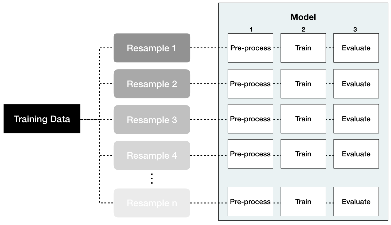
Figure 3.10: Performing feature engineering preprocessing within each resample helps to minimize data leakage.

For example, when standardizing numeric features, each resampled training data should use its own mean and variance estimates and these specific values should be applied to the same resampled test set. This imitates how real-life prediction occurs where we only know our current data’s mean and variance estimates; therefore, on new data that comes in where we need to predict we assume the feature values follow the same distribution of what we’ve seen in the past.

3.8.3 Putting the process together

To illustrate how this process works together via R code, let’s do a simple re-assessment on the ames data set that we did at the end of the last chapter (Section 2.7) and see if some simple feature engineering improves our prediction error. But first, we’ll formally introduce the recipes package, which we’ve been implicitly illustrating throughout.

The recipes package allows us to develop our feature engineering blueprint in a sequential nature. The idea behind recipes is similar to caret::preProcess() where we want to create the preprocessing blueprint but apply it later and within each resample.¹⁷

There are three main steps in creating and applying feature engineering with recipes:

recipe: where you define your feature engineering steps to create your blueprint.
prepare: estimate feature engineering parameters based on training data.
bake: apply the blueprint to new data.

The first step is where you define your blueprint (aka recipe). With this process, you supply the formula of interest (the target variable, features, and the data these are based on) with recipe() and then you sequentially add feature engineering steps with step_xxx(). For example, the following defines Sale_Price as the target variable and then uses all the remaining columns as features based on ames_train. We then:

Remove near-zero variance features that are categorical (aka nominal).
Ordinal encode our quality-based features (which are inherently ordinal).
Center and scale (i.e., standardize) all numeric features.
Perform dimension reduction by applying PCA to all numeric features.

blueprint <- recipe(Sale_Price ~ ., data = ames_train) %>%
  step_nzv(all_nominal())  %>%
  step_integer(matches("Qual|Cond|QC|Qu")) %>%
  step_center(all_numeric(), -all_outcomes()) %>%
  step_scale(all_numeric(), -all_outcomes()) %>%
  step_pca(all_numeric(), -all_outcomes())
  
blueprint
## Data Recipe
## 
## Inputs:
## 
##       role #variables
##    outcome          1
##  predictor         80
## 
## Operations:
## 
## Sparse, unbalanced variable filter on all_nominal
## Integer encoding for matches, Qual|Cond|QC|Qu
## Centering for all_numeric, -, all_outcomes()
## Scaling for all_numeric, -, all_outcomes()
## No PCA components were extracted.

Next, we need to train this blueprint on some training data. Remember, there are many feature engineering steps that we do not want to train on the test data (e.g., standardize and PCA) as this would create data leakage. So in this step we estimate these parameters based on the training data of interest.

prepare <- prep(blueprint, training = ames_train)
prepare
## Data Recipe
## 
## Inputs:
## 
##       role #variables
##    outcome          1
##  predictor         80
## 
## Training data contained 2053 data points and no missing data.
## 
## Operations:
## 
## Sparse, unbalanced variable filter removed Street, Alley, ... [trained]
## Integer encoding for Condition_1, Overall_Qual, Overall_Cond, ... [trained]
## Centering for Lot_Frontage, Lot_Area, ... [trained]
## Scaling for Lot_Frontage, Lot_Area, ... [trained]
## PCA extraction with Lot_Frontage, Lot_Area, ... [trained]

Lastly, we can apply our blueprint to new data (e.g., the training data or future test data) with bake().

baked_train <- bake(prepare, new_data = ames_train)
baked_test <- bake(prepare, new_data = ames_test)
baked_train
## # A tibble: 2,053 x 27
##    MS_SubClass MS_Zoning Lot_Shape Lot_Config Neighborhood Bldg_Type
##    <fct>       <fct>     <fct>     <fct>      <fct>        <fct>    
##  1 One_Story_… Resident… Slightly… Corner     North_Ames   OneFam   
##  2 One_Story_… Resident… Regular   Inside     North_Ames   OneFam   
##  3 One_Story_… Resident… Slightly… Corner     North_Ames   OneFam   
##  4 Two_Story_… Resident… Slightly… Inside     Gilbert      OneFam   
##  5 One_Story_… Resident… Regular   Inside     Stone_Brook  TwnhsE   
##  6 One_Story_… Resident… Slightly… Inside     Stone_Brook  TwnhsE   
##  7 Two_Story_… Resident… Regular   Inside     Gilbert      OneFam   
##  8 Two_Story_… Resident… Slightly… Corner     Gilbert      OneFam   
##  9 Two_Story_… Resident… Slightly… Inside     Gilbert      OneFam   
## 10 One_Story_… Resident… Regular   Inside     Gilbert      OneFam   
## # … with 2,043 more rows, and 21 more variables: House_Style <fct>,
## #   Roof_Style <fct>, Exterior_1st <fct>, Exterior_2nd <fct>,
## #   Mas_Vnr_Type <fct>, Foundation <fct>, Bsmt_Exposure <fct>,
## #   BsmtFin_Type_1 <fct>, Central_Air <fct>, Electrical <fct>,
## #   Garage_Type <fct>, Garage_Finish <fct>, Paved_Drive <fct>,
## #   Fence <fct>, Sale_Type <fct>, Sale_Price <int>, PC1 <dbl>, PC2 <dbl>,
## #   PC3 <dbl>, PC4 <dbl>, PC5 <dbl>

Consequently, the goal is to develop our blueprint, then within each resample iteration we want to apply prep() and bake() to our resample training and validation data. Luckily, the caret package simplifies this process. We only need to specify the blueprint and caret will automatically prepare and bake within each resample. We illustrate with the ames housing example.

First, we create our feature engineering blueprint to perform the following tasks:

Filter out near-zero variance features for categorical features.
Ordinally encode all quality features, which are on a 1–10 Likert scale.
Standardize (center and scale) all numeric features.
One-hot encode our remaining categorical features.

blueprint <- recipe(Sale_Price ~ ., data = ames_train) %>%
  step_nzv(all_nominal()) %>%
  step_integer(matches("Qual|Cond|QC|Qu")) %>%
  step_center(all_numeric(), -all_outcomes()) %>%
  step_scale(all_numeric(), -all_outcomes()) %>%
  step_dummy(all_nominal(), -all_outcomes(), one_hot = TRUE)

Next, we apply the same resampling method and hyperparameter search grid as we did in Section 2.7. The only difference is when we train our resample models with train(), we supply our blueprint as the first argument and then caret takes care of the rest.

# Specify resampling plan
cv <- trainControl(
  method = "repeatedcv", 
  number = 10, 
  repeats = 5
)

# Construct grid of hyperparameter values
hyper_grid <- expand.grid(k = seq(2, 25, by = 1))

# Tune a knn model using grid search
knn_fit2 <- train(
  blueprint, 
  data = ames_train, 
  method = "knn", 
  trControl = cv, 
  tuneGrid = hyper_grid,
  metric = "RMSE"
)

Looking at our results we see that the best model was associated with $k=$ 13, which resulted in a cross-validated RMSE of 32,898. Figure 3.11 illustrates the cross-validated error rate across the spectrum of hyperparameter values that we specified.

# print model results
knn_fit2
## k-Nearest Neighbors 
## 
## 2053 samples
##   80 predictor
## 
## Recipe steps: nzv, integer, center, scale, dummy 
## Resampling: Cross-Validated (10 fold, repeated 5 times) 
## Summary of sample sizes: 1848, 1849, 1848, 1847, 1848, 1848, ... 
## Resampling results across tuning parameters:
## 
##   k   RMSE      Rsquared   MAE     
##    2  36067.27  0.8031344  22618.51
##    3  34924.85  0.8174313  21726.77
##    4  34515.13  0.8223547  21281.38
##    5  34040.72  0.8306678  20968.31
##    6  33658.36  0.8366193  20850.36
##    7  33477.81  0.8411600  20728.86
##    8  33272.66  0.8449444  20607.91
##    9  33151.51  0.8473631  20542.64
##   10  33018.91  0.8496265  20540.82
##   11  32963.31  0.8513253  20565.32
##   12  32931.68  0.8531010  20615.63
##   13  32898.37  0.8545475  20621.94
##   14  32916.05  0.8554991  20660.38
##   15  32911.62  0.8567444  20721.47
##   16  32947.41  0.8574756  20771.31
##   17  33012.23  0.8575633  20845.23
##   18  33056.07  0.8576921  20942.94
##   19  33152.81  0.8574236  21038.13
##   20  33243.06  0.8570209  21125.38
##   21  33300.40  0.8566910  21186.67
##   22  33332.59  0.8569302  21240.79
##   23  33442.28  0.8564495  21325.81
##   24  33464.31  0.8567895  21345.11
##   25  33514.23  0.8568821  21375.29
## 
## RMSE was used to select the optimal model using the smallest value.
## The final value used for the model was k = 13.

# plot cross validation results
ggplot(knn_fit2)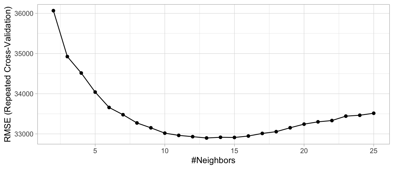

Figure 3.11: Results from the same grid search performed in Section 2.7 but with feature engineering performed within each resample.

By applying a handful of the preprocessing techniques discussed throughout this chapter, we were able to reduce our prediction error by over $10,000. The chapters that follow will look to see if we can continue reducing our error by applying different algorithms and feature engineering blueprints.

References

Box, George EP, and David R Cox. 1964. “An Analysis of Transformations.” Journal of the Royal Statistical Society. Series B (Methodological). JSTOR, 211–52.

Breiman, Leo, and others. 2001. “Statistical Modeling: The Two Cultures (with Comments and a Rejoinder by the Author).” Statistical Science 16 (3). Institute of Mathematical Statistics: 199–231.

Carroll, Raymond J, and David Ruppert. 1981. “On Prediction and the Power Transformation Family.” Biometrika 68 (3). Oxford University Press: 609–15.

Chollet, François, and Joseph J Allaire. 2018. Deep Learning with R. Manning Publications Company.

Gower, John C. 1971. “A General Coefficient of Similarity and Some of Its Properties.” Biometrics. JSTOR, 857–71.

Granitto, Pablo M, Cesare Furlanello, Franco Biasioli, and Flavia Gasperi. 2006. “Recursive Feature Elimination with Random Forest for Ptr-Ms Analysis of Agroindustrial Products.” Chemometrics and Intelligent Laboratory Systems 83 (2). Elsevier: 83–90.

Guo, Cheng, and Felix Berkhahn. 2016. “Entity Embeddings of Categorical Variables.” arXiv Preprint arXiv:1604.06737.

Kuhn, Max, and Kjell Johnson. 2013. Applied Predictive Modeling. Vol. 26. Springer.

Kuhn, Max, and Kjell Johnson. 2019. Feature Engineering and Selection: A Practical Approach for Predictive Models. Chapman & Hall/CRC.

Kursa, Miron B, Witold R Rudnicki, and others. 2010. “Feature Selection with the Boruta Package.” J Stat Softw 36 (11): 1–13.

Little, Roderick JA, and Donald B Rubin. 2014. Statistical Analysis with Missing Data. Vol. 333. John Wiley & Sons.

Maldonado, Sebastián, and Richard Weber. 2009. “A Wrapper Method for Feature Selection Using Support Vector Machines.” Information Sciences 179 (13). Elsevier: 2208–17.

Micci-Barreca, Daniele. 2001. “A Preprocessing Scheme for High-Cardinality Categorical Attributes in Classification and Prediction Problems.” ACM SIGKDD Explorations Newsletter 3 (1). ACM: 27–32.

Saeys, Yvan, Iñaki Inza, and Pedro Larrañaga. 2007. “A Review of Feature Selection Techniques in Bioinformatics.” Bioinformatics 23 (19). Oxford University Press: 2507–17.

Shah, Anoop D, Jonathan W Bartlett, James Carpenter, Owen Nicholas, and Harry Hemingway. 2014. “Comparison of Random Forest and Parametric Imputation Models for Imputing Missing Data Using Mice: A Caliber Study.” American Journal of Epidemiology 179 (6). Oxford University Press: 764–74.

Stekhoven, Daniel J. 2015. “MissForest: Nonparametric Missing Value Imputation Using Random Forest.” Astrophysics Source Code Library.

Tierney, Nicholas. 2019. Visdat: Preliminary Visualisation of Data. https://CRAN.R-project.org/package=visdat.

West, Brady T, Kathleen B Welch, and Andrzej T Galecki. 2014. Linear Mixed Models: A Practical Guide Using Statistical Software. Chapman; Hall/CRC.

Zheng, Alice, and Amanda Casari. 2018. Feature Engineering for Machine Learning: Principles and Techniques for Data Scientists. O’Reilly Media, Inc.

Zumel, Nina, and John Mount. 2016. “Vtreat: A Data. Frame Processor for Predictive Modeling.” arXiv Preprint arXiv:1611.09477.

https://www.kaggle.com/c/house-prices-advanced-regression-techniques ↩
https://github.com/Quartz/bad-data-guide ↩
Little and Rubin (2014) discuss two different kinds of missingness at random; however, we combine them for simplicity as their nuanced differences are distinguished between the two in practice.↩
If your data set is large, deleting missing observations that have missing values at random rarely impacts predictive performance. However, as your data sets get smaller, preserving observations is critical and alternative solutions should be explored.↩
For example, standardizing numeric features will include the imputed numeric values in the calculation and one-hot encoding will include the imputed categorical value.↩
See Kuhn and Johnson (2013) Section 19.1 for data set generation.↩
In fact, most of the feature engineering capabilities found in resample can also be found in caret::preProcess().↩