Chapter 22 Model-based Clustering

Traditional clustering algorithms such as k-means (Chapter 20) and hierarchical (Chapter 21) clustering are heuristic-based algorithms that derive clusters directly based on the data rather than incorporating a measure of probability or uncertainty to the cluster assignments. Model-based clustering attempts to address this concern and provide soft assignment where observations have a probability of belonging to each cluster. Moreover, model-based clustering provides the added benefit of automatically identifying the optimal number of clusters. This chapter covers Gaussian mixture models, which are one of the most popular model-based clustering approaches available.

22.1 Prerequisites

For this chapter we’ll use the following packages with the emphasis on mclust (Fraley, Raftery, and Scrucca 2019):

# Helper packages
library(dplyr)    # for data manipulation
library(ggplot2)  # for data visualization

# Modeling packages
library(mclust)   # for fitting clustering algorithms

To illustrate the main concepts of model-based clustering we’ll use the geyser data provided by the MASS package along with the my_basket data.

data(geyser, package = 'MASS')

url <- "https://koalaverse.github.io/homlr/data/my_basket.csv"
my_basket <- readr::read_csv(url)

22.2 Measuring probability and uncertainty

The key idea behind model-based clustering is that the data are considered as coming from a mixture of underlying probability distributions. The most popular approach is the Gaussian mixture model (GMM) (Banfield and Raftery 1993) where each observation is assumed to be distributed as one of \(k\) multivariate-normal distributions, where \(k\) is the number of clusters (commonly referred to as components in model-based clustering). For a comprehensive review of model-based clustering, see Fraley and Raftery (2002).

GMMs are founded on the multivariate normal (Gaussian) distribution where \(p\) variables (\(X_1, X_2, \dots, X_p\)) are assumed to have means \(\mu = \left(\mu_1, \mu_2, \dots, \mu_p\right)\) and a covariance matrix \(\Sigma\), which describes the joint variability (i.e., covariance) between each pair of variables:

\[\begin{equation} \tag{22.1} \sum = \left[\begin{array}{cccc} \sigma_{1}^{2} & \sigma_{1, 2} & \cdots & \sigma_{1, p} \\ \sigma_{2, 1} & \sigma_{2}^{2} & \cdots & \sigma_{2, p} \\ \vdots & \vdots & \ddots & \vdots \\ \sigma_{p, 1} & \sigma_{p, 2}^{2} & \cdots & \sigma_{p}^{2} \end{array}\right]. \end{equation}\]

Note that \(\Sigma\) contains \(p\) variances (\(\sigma_1^2, \sigma_2^2, \dots, \sigma_p^2\)) and \(p\left(p - 1\right) / 2\) unique covariances \(\sigma_{i, j}\) (\(i \ne j\)); note that \(\sigma_{i, j} = \sigma_{j, i}\). A multivariate-normal distribution with mean \(\mu\) and covariance \(|sigma\) is notationally represented by Equation (22.2):

\[\begin{equation} \tag{22.2} \left(X_1, X_2, \dots, X_p\right) \sim N_p \left( \mu, \Sigma \right). \end{equation}\]

This distribution has the property that every subset of variables (say, \(X_1\), \(X_5\), and \(X_9\)) also has a multivariate normal distribution (albeit with a different mean and covariance structure). GMMs assume the clusters can be created using \(k\) Gaussian distributions. For example, if there are two variables (say, \(X\) and \(Y\)), then each observation \(\left(X_i, Y_i\right)\) is modeled has having been sampled from one of \(k\) distributions (\(N_1\left(\mu_1, \Sigma_1 \right), N_2\left(\mu_2, \Sigma_2 \right), \dots, N_p\left(\mu_p, \Sigma_p \right)\)). This is illustrated in Figure 22.1 which suggests variables \(X\) and \(Y\) come from three multivariate distributions. However, as the data points deviate from the center of one of the three clusters, the probability that they align to a particular cluster decreases as indicated by the fading elliptical rings around each cluster center.

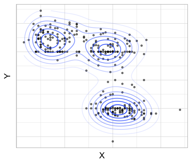
Figure 22.1: Data points across two features (X and Y) appear to come from three multivariate normal distributions.

We can illustrate this concretely by applying a GMM model to the geyser data, which is the data illustrated in Figure 22.1. To do so we apply Mclust() and specify three components. Plotting the output (Figure 22.2) provides a density plot (left) just like we saw in Figure 22.1 and the component assignment for each observation based on the largest probability (right). In the uncertainty plot (right), you’ll notice the observations near the center of the densities are small, indicating small uncertainty (or high probability) of being from that respective component; however, the observations that are large represent observations with high uncertainty (or low probability) regarding the component they are aligned to.

# Apply GMM model with 3 components
geyser_mc <- Mclust(geyser, G = 3)

# Plot results
plot(geyser_mc, what = "density")
plot(geyser_mc, what = "uncertainty")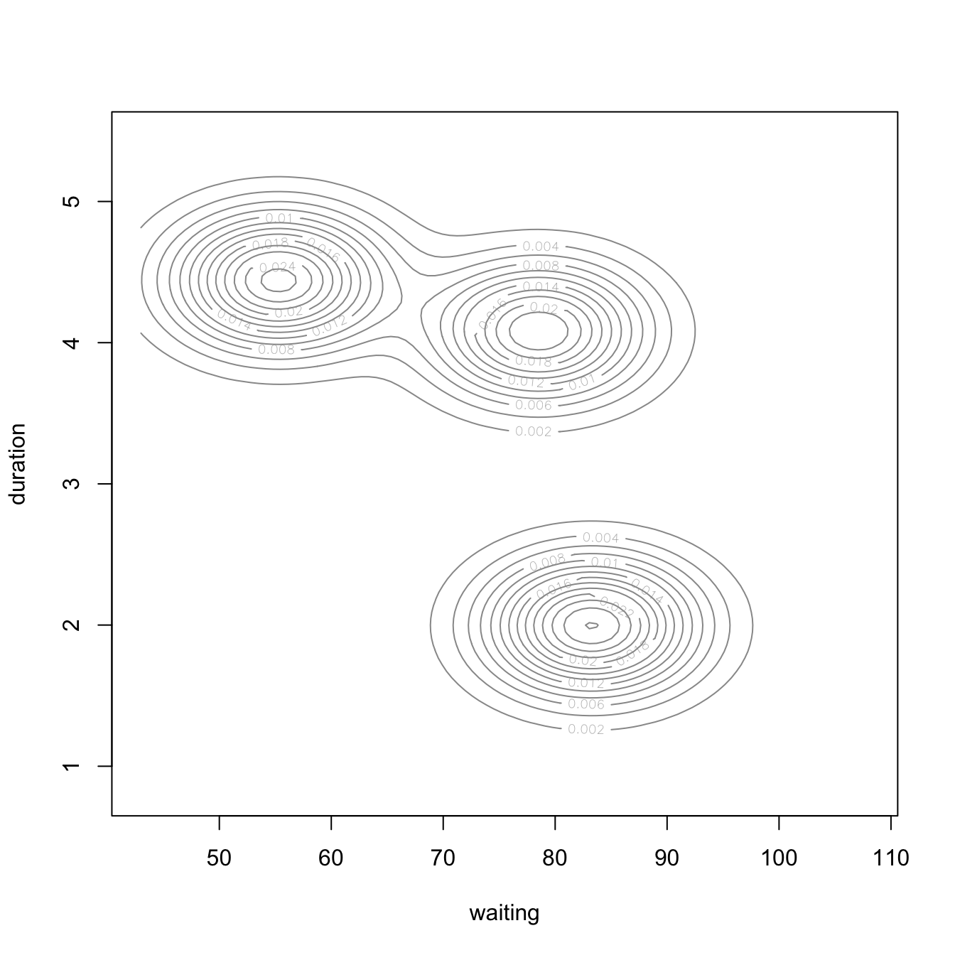

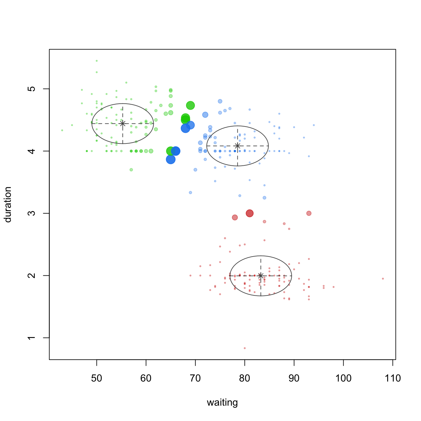
Figure 22.2: Multivariate density plot (left) highlighting three clusters in the geyser data and an uncertainty plot (right) highlighting observations with high uncertainty of which cluster they are a member of.

This idea of a probabilistic cluster assignment can be quite useful as it allows you to identify observations with high or low cluster uncertainty and, potentially, target them uniquely or provide alternative solutions. For example, the following six observations all have nearly 50% probability of being assigned to two different clusters. If this were an advertising data set and you were marketing to these observations you may want to provide them with a combination of marketing solutions for the two clusters they are nearest to. Or you may want to perform additional A/B testing on them to try gain additional confidence regarding which cluster they align to most.

# Observations with high uncertainty
sort(geyser_mc$uncertainty, decreasing = TRUE) %>% head()
##       187       211        85       285        28       206 
## 0.4689087 0.4542588 0.4355496 0.4355496 0.4312406 0.4168440

22.3 Covariance types

The covariance matrix in Equation (22.1) describes the geometry of the clusters; namely, the volume, shape, and orientation of the clusters. Looking at Figure 22.2, the clusters and their densities appear approximately proportional in size and shape. However, this is not a requirement of GMMs. In fact, GMMs allow for far more flexible clustering structures.

This is done by adding constraints to the covariance matrix \(\Sigma\). These constraints can be one or more of the following:

1. volume: each cluster has approximately the same number of observations;
2. shape: each cluster has approximately the same variance so that the distribution is spherical;
3. orientation: each cluster is forced to be axis-aligned.

The various combinations of the above constraints have been classified into three main families of models: spherical, diagonal, and general (also referred to as ellipsoidal) families (Celeux and Govaert 1995). These combinations are listed in Table 22.1. See Fraley et al. (2012) regarding the technical implementation of these covariance parameters.

Table 22.1: Parameterizations of the covariance matrix

Model	Family	Volume	Shape	Orientation	Identifier
1	Spherical	Equal	Equal	NA	EII
2	Spherical	Variable	Equal	NA	VII
3	Diagonal	Equal	Equal	Axes	EEI
4	Diagonal	Variable	Equal	Axes	VEI
5	Diagonal	Equal	Variable	Axes	EVI
6	Diagonal	Variable	Variable	Axes	VVI
7	General	Equal	Equal	Equal	EEE
8	General	Equal	Variable	Equal	EVE
9	General	Variable	Equal	Equal	VEE
10	General	Variable	Variable	Equal	VVE
11	General	Equal	Equal	Variable	EEV
12	General	Variable	Equal	Variable	VEV
13	General	Equal	Variable	Variable	EVV
14	General	Variable	Variable	Variable	VVV

These various covariance parameters allow GMMs to capture unique clustering structures in data, as illustrated in Figure 22.3.

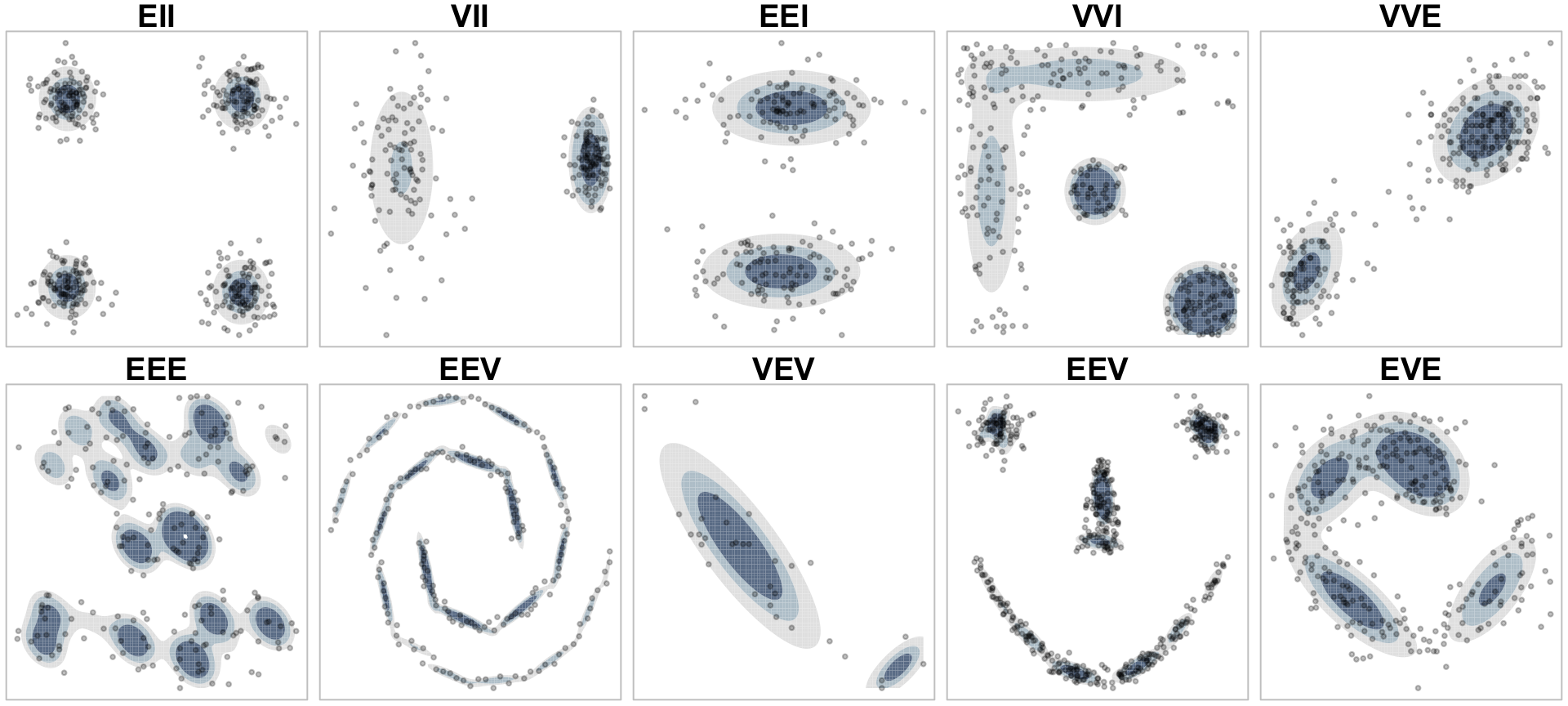
Figure 22.3: Graphical representation of how different covariance models allow GMMs to capture different cluster structures.

Users can optionally specify a conjugate prior if prior knowledge of the underlying probability distributions are available. By default, Mclust() does not apply a prior for modeling.

22.4 Model selection

If we assess the summary of our geyser_mc model we see that, behind the scenes, Mclust() applied the EEI model.

A more detailed summary, including the estimated parameters, can be obtained using summary(geyser_mc, parameters = TRUE).

summary(geyser_mc)
## ---------------------------------------------------- 
## Gaussian finite mixture model fitted by EM algorithm 
## ---------------------------------------------------- 
## 
## Mclust EEI (diagonal, equal volume and shape) model with 3 components: 
## 
##  log-likelihood   n df      BIC       ICL
##       -1371.823 299 10 -2800.65 -2814.577
## 
## Clustering table:
##   1   2   3 
##  91 107 101

However, Mclust() will apply all 14 models from Table 22.3 and identify the one that best characterizes the data. To select the optimal model, any model selection procedure can be applied (e.g., Akaike information criteria (AIC), likelihood ratio, etc.); however, the Bayesian information criterion (BIC) has been shown to work well in model-based clustering (Dasgupta and Raftery 1998; Fraley and Raftery 1998) and is typically the default. Mclust() implements BIC as represented in Equation (22.3)

\[\begin{equation} \tag{22.3} BIC = -2\log\left(L\right) + m \log\left(n\right), \end{equation}\]

where \(\log\left(n\right)\) is the maximized loglikelihood for the model and data, \(m\) is the number of free parameters to be estimated in the given model, and \(n\) is the number observations in the data. This penalizes large models with many clusters.

The objective in hyperparameter tuning with Mclust() is to maximize BIC.

Not only can we use BIC to identify the optimal covariance parameters, but we can also use it to identify the optimal number of clusters. Rather than specify G = 3 in Mclust(), leaving G = NULL forces Mclust() to evaluate 1–9 clusters and select the optimal number of components based on BIC. Alternatively, you can specify certain values to evaluate for G. The following performs a hyperparameter search across all 14 covariance models for 1–9 clusters on the geyser data. The left plot in Figure 22.4 shows that the EEI and VII models perform particularly poor while the rest of the models perform much better and have little differentiation. The optimal model uses the VVI covariance parameters, which identified four clusters and has a BIC of -2768.568.

geyser_optimal_mc <- Mclust(geyser)

summary(geyser_optimal_mc)
## ---------------------------------------------------- 
## Gaussian finite mixture model fitted by EM algorithm 
## ---------------------------------------------------- 
## 
## Mclust VVI (diagonal, varying volume and shape) model with 4 components: 
## 
##  log-likelihood   n df       BIC       ICL
##        -1330.13 299 19 -2768.568 -2798.746
## 
## Clustering table:
##  1  2  3  4 
## 90 17 98 94

legend_args <- list(x = "bottomright", ncol = 5)
plot(geyser_optimal_mc, what = 'BIC', legendArgs = legend_args)
plot(geyser_optimal_mc, what = 'classification')
plot(geyser_optimal_mc, what = 'uncertainty')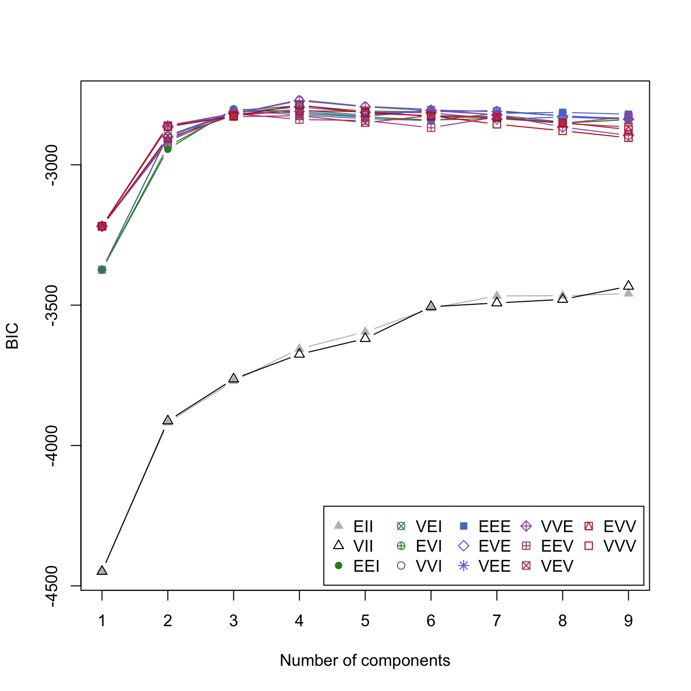

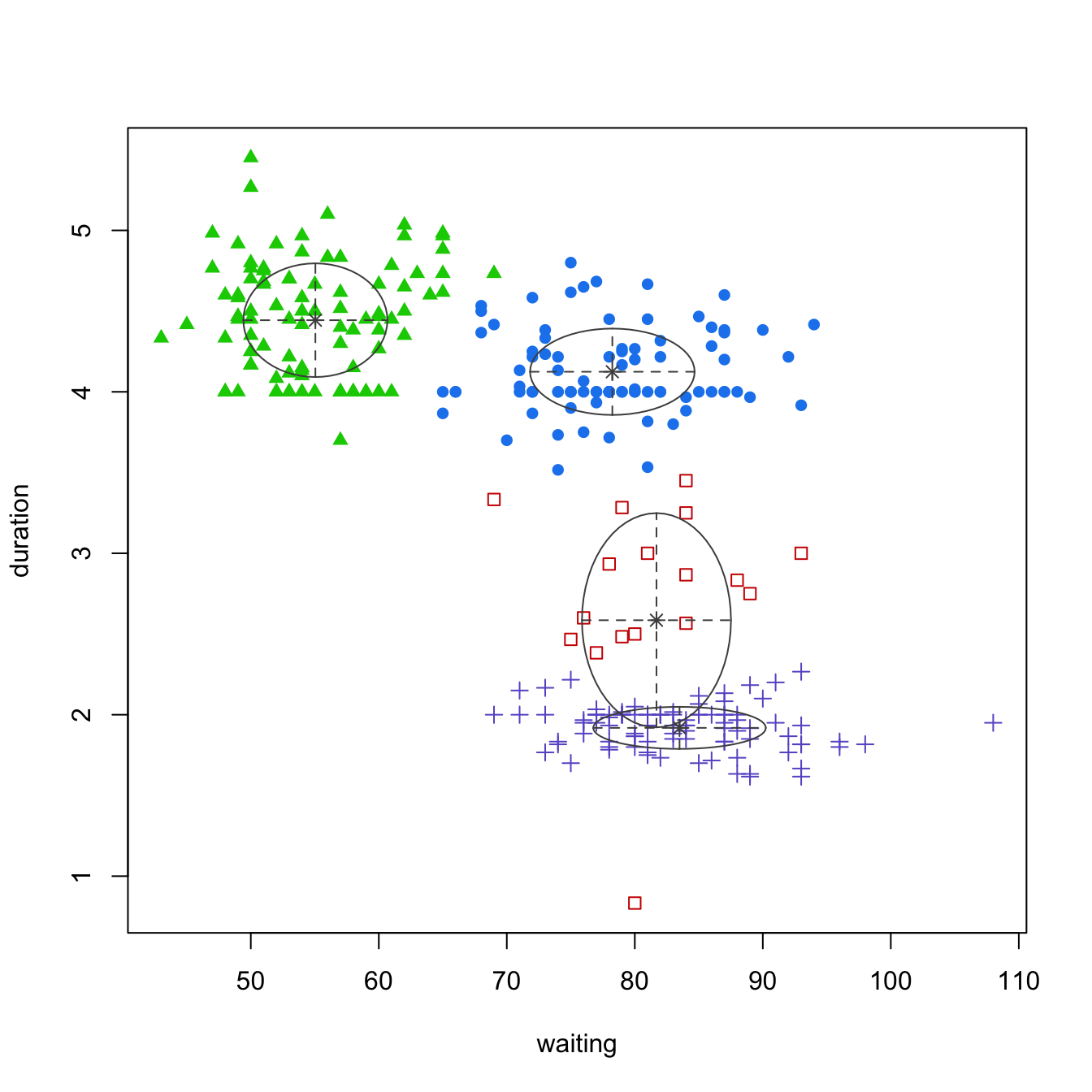
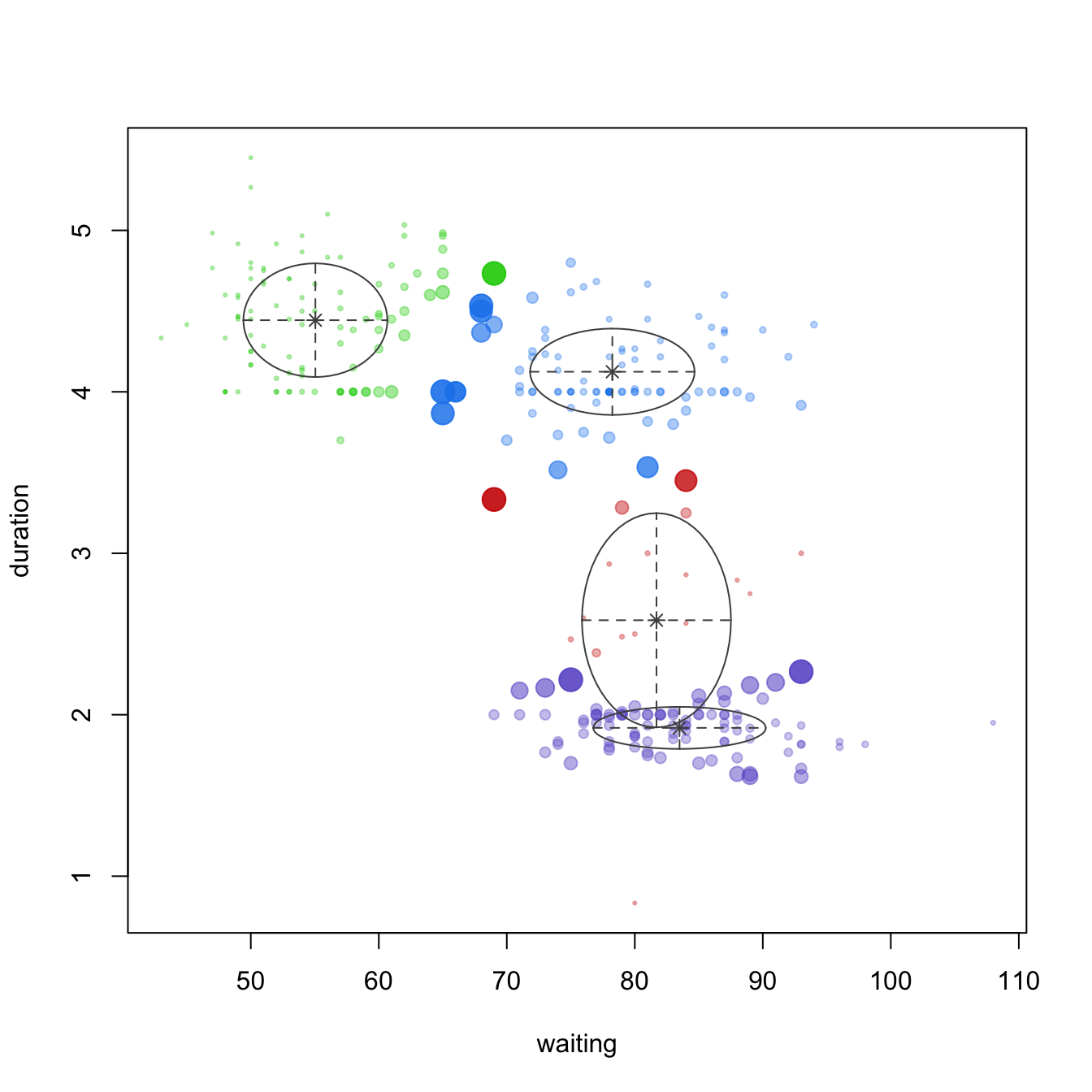
Figure 22.4: Identifying the optimal GMM model and number of clusters for the geyser data (left). The classification (center) and uncertainty (right) plots illustrate which observations are assigned to each cluster and their level of assignment uncertainty.

22.5 My basket example

Let’s turn to our my_basket data to demonstrate GMMs on a more modern sized data set. The following performs a search across all 14 GMM models and across 1–20 clusters. If you are following along and running the code you’ll notice that GMMs are computationally slow, especially since they are assessing 14 models for each cluster size instance. This GMM hyperparameter search took a little over a minute. Figure 22.5 illustrates the BIC scores and we see that the optimal GMM method is EEV with six clusters.

You may notice that not all models generate results for each cluster size (e.g., the VVI model only produced results for clusters 1–3). This is because the model could not converge on optimal results for those settings. This becomes more problematic as data sets get larger. Often, performing dimension reduction prior to a GMM can minimize this issue.

my_basket_mc <- Mclust(my_basket, 1:20)

summary(my_basket_mc)
## ---------------------------------------------------- 
## Gaussian finite mixture model fitted by EM algorithm 
## ---------------------------------------------------- 
## 
## Mclust EEV (ellipsoidal, equal volume and shape) model with 6 components: 
## 
##  log-likelihood    n   df      BIC       ICL
##        8308.915 2000 5465 -24921.1 -25038.38
## 
## Clustering table:
##   1   2   3   4   5   6 
## 391 403  75 315 365 451

plot(my_basket_mc, what = 'BIC', 
     legendArgs = list(x = "bottomright", ncol = 5))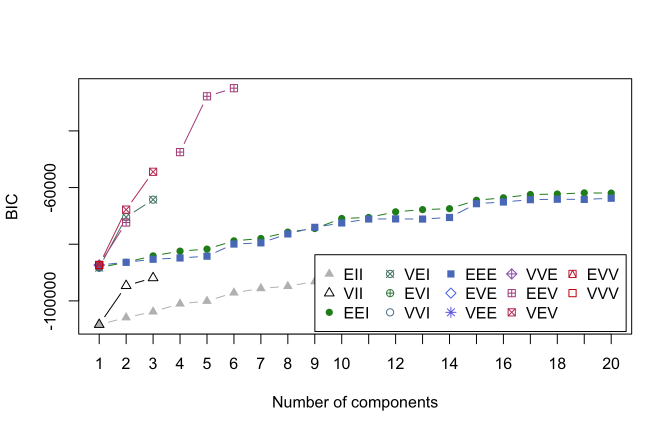

Figure 22.5: BIC scores for clusters (components) ranging from 1-20

We can look across our six clusters and assess the probabilities of cluster membership. Figure 22.6 illustrates very bimodal distributions of probabilities. Observations with greater than 0.50 probability will be aligned to a given cluster so this bimodality is preferred as it illustrates that observations have either a very high probability of the cluster they are aligned to or a very low probability, which means they would not be aligned to that cluster.

Looking at cluster C3, we see that there are very few, if any, observations in the middle of the probability range. C3 also has far fewer observations with high probability. This means that C3 is the smallest of the clusters (confirmed using summary(my_basket_mc)) above, and that C3 is a more compact cluster. As clusters have more observations with middling levels of probability (i.e., 0.25–0.75), their clusters are usually less compact. Therefore, cluster C2 is less compact than cluster C3.

probabilities <- my_basket_mc$z 
colnames(probabilities) <- paste0('C', 1:6)

probabilities <- probabilities %>%
  as.data.frame() %>%
  mutate(id = row_number()) %>%
  tidyr::gather(cluster, probability, -id)

ggplot(probabilities, aes(probability)) +
  geom_histogram() +
  facet_wrap(~ cluster, nrow = 2)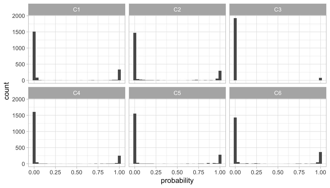

Figure 22.6: Distribution of probabilities for all observations aligning to each of the six clusters.

We can extract the cluster membership for each observation with my_basket_mc$classification. In Figure 22.7 we find the observations that are aligned to each cluster but the uncertainty of their membership to that particular cluster is 0.25 or greater. You may notice that cluster three is not represented. Recall from Figure 22.6 that cluster three’s observations all had very strong membership probabilities so they have no observations with uncertainty greater than 0.25.

uncertainty <- data.frame(
  id = 1:nrow(my_basket),
  cluster = my_basket_mc$classification,
  uncertainty = my_basket_mc$uncertainty
)

uncertainty %>%
  group_by(cluster) %>%
  filter(uncertainty > 0.25) %>%
  ggplot(aes(uncertainty, reorder(id, uncertainty))) +
  geom_point() +
  facet_wrap(~ cluster, scales = 'free_y', nrow = 1)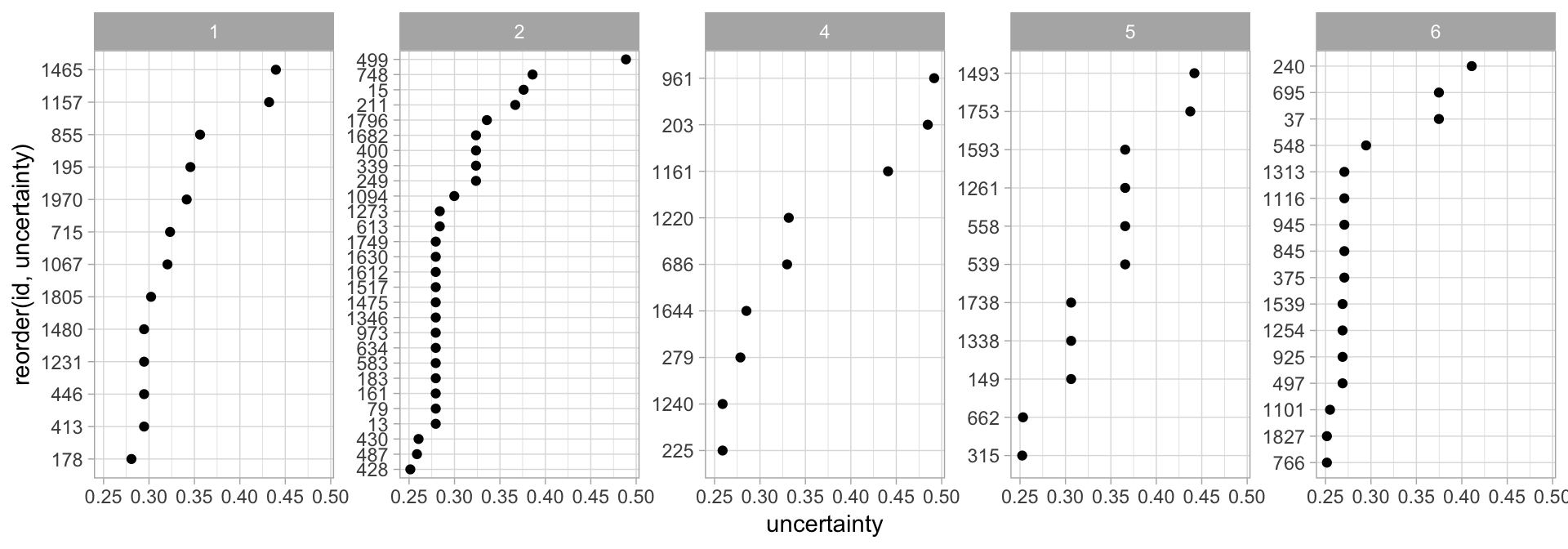

Figure 22.7: Observations that are aligned to each cluster but their uncertainty of membership is greater than 0.25.

When doing cluster analysis, our goal is to find those observations that are most similar to others. What defines this similarity becomes difficult as our data sets become larger. Let’s take a look at cluster two. The following standardizes the count of each product across all baskets and then looks at consumption for cluster two. Figure 22.8 illustrates the results and shows that cluster two baskets have above average consumption for candy bars, lottery tickets, cigarettes, and alcohol.

Needless to say, this group may include our more unhealthy baskets—or maybe they’re the recreational baskets made on the weekends when people just want to sit on the deck and relax with a drink in one hand and a candy bar in the other! Regardless, this group is likely to receive marketing ads for candy bars, alcohol, and the like rather than the items we see at the bottom of Figure 22.8, which represent the items this group consumes less than the average observations.

cluster2 <- my_basket %>%
  scale() %>%
  as.data.frame() %>%
  mutate(cluster = my_basket_mc$classification) %>%
  filter(cluster == 2) %>%
  select(-cluster)

cluster2 %>%
  tidyr::gather(product, std_count) %>%
  group_by(product) %>%
  summarize(avg = mean(std_count)) %>%
  ggplot(aes(avg, reorder(product, avg))) +
  geom_point() +
  labs(x = "Average standardized consumption", y = NULL)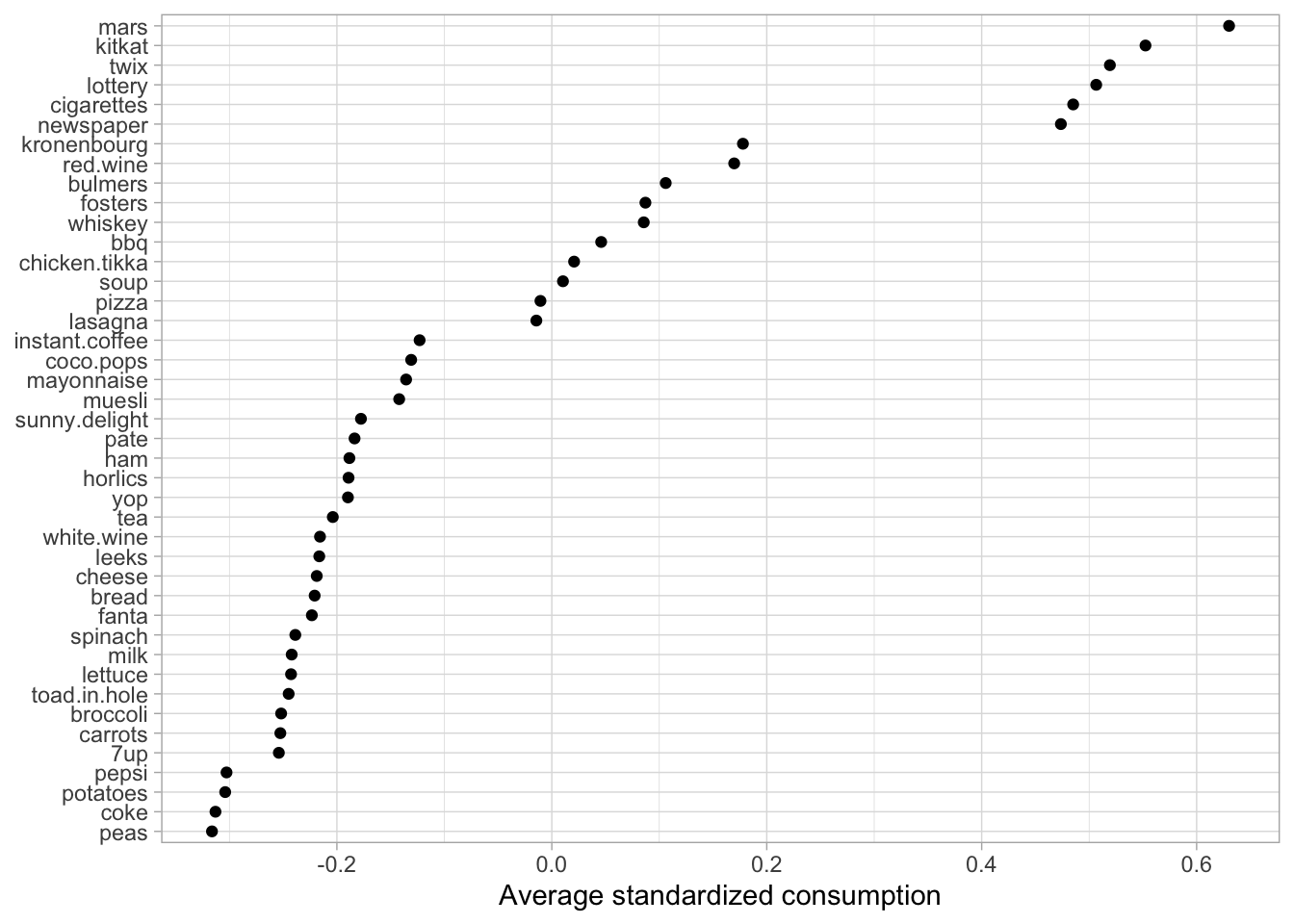

Figure 22.8: Average standardized consumption for cluster 2 observations compared to all observations.

22.6 Final thoughts

Model-based clustering techniques do have their limitations. The methods require an underlying model for the data (e.g., GMMs assume multivariate normality), and the cluster results are heavily dependent on this assumption. Although there have been many advancements to limit this constraint (Lee and McLachlan 2013), software implementations are still lacking.

A more significant limitation is the computational demands. Classical model-based clustering show disappointing computational performance in high-dimensional spaces (Bouveyron and Brunet-Saumard 2014). This is mainly due to the fact that model-based clustering methods are dramatically over-parameterized. The primary approach for dealing with this is to perform dimension reduction prior to clustering. Although this often improves computational performance, reducing the dimension without taking into consideration the clustering goal may be dangerous. Indeed, dimension reduction may yield a loss of information which could have been useful for discriminating the groups. There have been alternative solutions proposed, such as high-dimensional GMMs (Bouveyron, Girard, and Schmid 2007), which has been implemented in the HDclassif package (Berge, Bouveyron, and Girard 2018).

References

Banfield, Jeffrey D, and Adrian E Raftery. 1993. “Model-Based Gaussian and Non-Gaussian Clustering.” Biometrics. JSTOR, 803–21.

Berge, Laurent, Charles Bouveyron, and Stephane Girard. 2018. HDclassif: High Dimensional Supervised Classification and Clustering. https://CRAN.R-project.org/package=HDclassif.

Bouveyron, Charles, and Camille Brunet-Saumard. 2014. “Model-Based Clustering of High-Dimensional Data: A Review.” Computational Statistics & Data Analysis 71. Elsevier: 52–78.

Bouveyron, Charles, Stéphane Girard, and Cordelia Schmid. 2007. “High-Dimensional Data Clustering.” Computational Statistics & Data Analysis 52 (1). Elsevier: 502–19.

Celeux, Gilles, and Gérard Govaert. 1995. “Gaussian Parsimonious Clustering Models.” Pattern Recognition 28 (5). Elsevier: 781–93.

Dasgupta, Abhijit, and Adrian E Raftery. 1998. “Detecting Features in Spatial Point Processes with Clutter via Model-Based Clustering.” Journal of the American Statistical Association 93 (441). Taylor & Francis: 294–302.

Fraley, Chris, and Adrian E Raftery. 1998. “How Many Clusters? Which Clustering Method? Answers via Model-Based Cluster Analysis.” The Computer Journal 41 (8). Oxford University Press: 578–88.

Fraley, Chris, and Adrian E Raftery. 2002. “Model-Based Clustering, Discriminant Analysis, and Density Estimation.” Journal of the American Statistical Association 97 (458). Taylor & Francis: 611–31.

Fraley, Chris, Adrian E Raftery, T Brendan Murphy, and Luca Scrucca. 2012. “Mclust Version 4 for R: Normal Mixture Modeling for Model-Based Clustering, Classification, and Density Estimation.” University of Washington.

Fraley, Chris, Adrian E. Raftery, and Luca Scrucca. 2019. Mclust: Gaussian Mixture Modelling for Model-Based Clustering, Classification, and Density Estimation. https://CRAN.R-project.org/package=mclust.

Lee, Sharon X, and Geoffrey J McLachlan. 2013. “Model-Based Clustering and Classification with Non-Normal Mixture Distributions.” Statistical Methods & Applications 22 (4). Springer: 427–54.