Chapter 8 K-Nearest Neighbors

K-nearest neighbor (KNN) is a very simple algorithm in which each observation is predicted based on its “similarity” to other observations. Unlike most methods in this book, KNN is a memory-based algorithm and cannot be summarized by a closed-form model. This means the training samples are required at run-time and predictions are made directly from the sample relationships. Consequently, KNNs are also known as lazy learners (Cunningham and Delany 2007) and can be computationally inefficient. However, KNNs have been successful in a large number of business problems (see, for example, Jiang et al. (2012) and Mccord and Chuah (2011)) and are useful for preprocessing purposes as well (as was discussed in Section 3.3.2).

8.1 Prerequisites

For this chapter we’ll use the following packages:

# Helper packages
library(dplyr)      # for data wrangling
library(ggplot2)    # for awesome graphics
library(rsample)    # for creating validation splits
library(recipes)    # for feature engineering

# Modeling packages
library(caret)       # for fitting KNN models

To illustrate various concepts we’ll continue working with the ames_train and ames_test data sets created in Section 2.7; however, we’ll also illustrate the performance of KNNs on the employee attrition and MNIST data sets.

# create training (70%) set for the rsample::attrition data.
attrit <- attrition %>% mutate_if(is.ordered, factor, ordered = FALSE)
set.seed(123)
churn_split <- initial_split(attrit, prop = .7, strata = "Attrition")
churn_train <- training(churn_split)

# import MNIST training data
mnist <- dslabs::read_mnist()
names(mnist)
## [1] "train" "test"

8.2 Measuring similarity

The KNN algorithm identifies \(k\) observations that are “similar” or nearest to the new record being predicted and then uses the average response value (regression) or the most common class (classification) of those \(k\) observations as the predicted output.

For illustration, consider our Ames housing data. In real estate, Realtors determine what price they will list (or market) a home for based on “comps” (comparable homes). To identify comps, they look for homes that have very similar attributes to the one being sold. This can include similar features (e.g., square footage, number of rooms, and style of the home), location (e.g., neighborhood and school district), and many other attributes. The Realtor will look at the typical sale price of these comps and will usually list the new home at a very similar price to the prices these comps sold for.

As an example, Figure 8.1 maps 10 homes (blue) that are most similar to the home of interest (red). These homes are all relatively close to the target home and likely have similar characteristics (e.g., home style, size, and school district). Consequently, the Realtor would likely list the target home around the average price that these comps sold for. In essence, this is what the KNN algorithm will do.

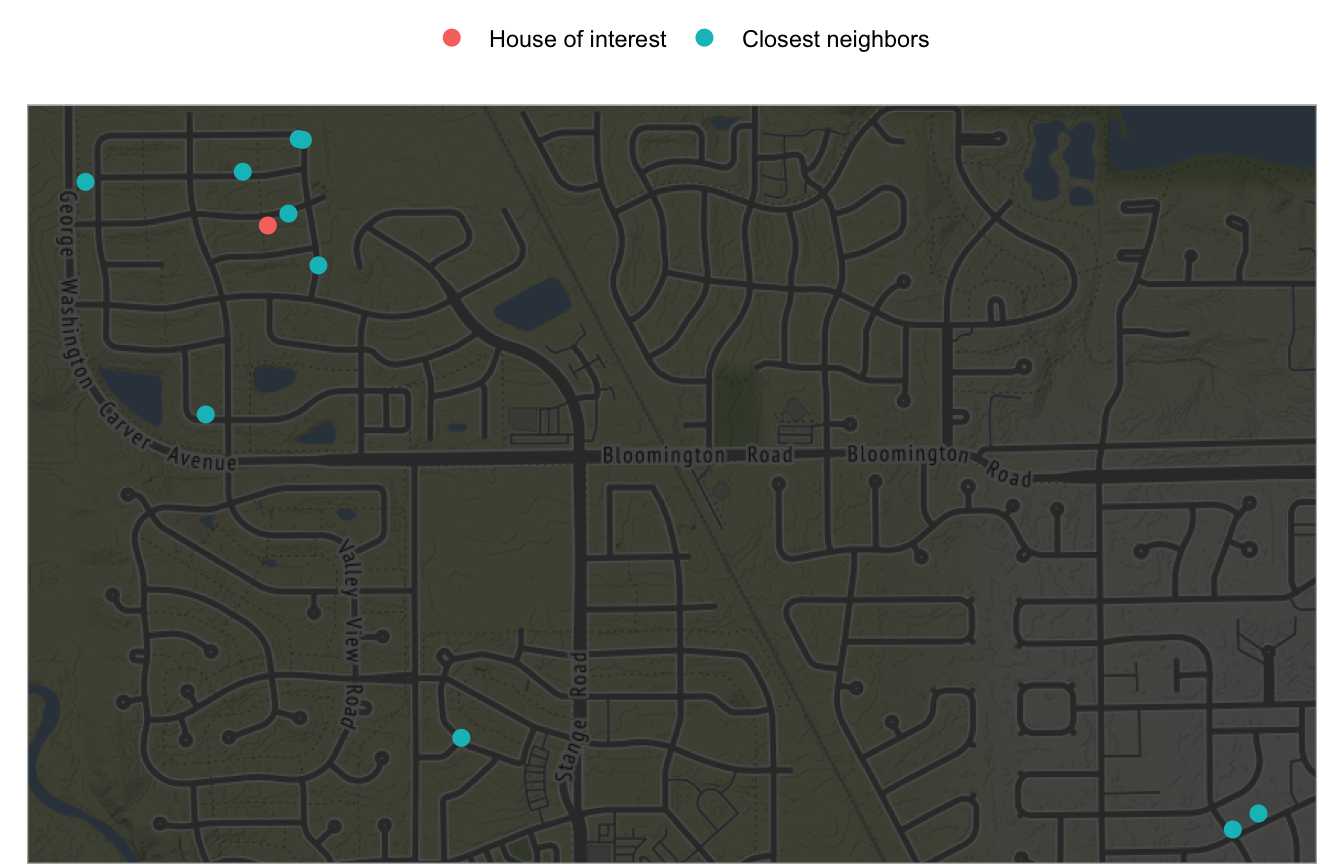
Figure 8.1: The 10 nearest neighbors (blue) whose home attributes most closely resemble the house of interest (red).

8.2.1 Distance measures

How do we determine the similarity between observations (or homes as in Figure 8.1)? We use distance (or dissimilarity) metrics to compute the pairwise differences between observations. The most common distance measures are the Euclidean (8.1) and Manhattan (8.2) distance metrics; both of which measure the distance between observation \(x_a\) and \(x_b\) for all \(j\) features.

\[\begin{equation} \tag{8.1} \sqrt{\sum^P_{j=1}(x_{aj} - x_{bj})^2} \end{equation}\]

\[\begin{equation} \tag{8.2} \sum^P_{j=1} | x_{aj} - x_{bj} | \end{equation}\]

Euclidean distance is the most common and measures the straight-line distance between two samples (i.e., how the crow flies). Manhattan measures the point-to-point travel time (i.e., city block) and is commonly used for binary predictors (e.g., one-hot encoded 0/1 indicator variables). A simplified example is presented below and illustrated in Figure 8.2 where the distance measures are computed for the first two homes in ames_train and for only two features (Gr_Liv_Area & Year_Built).

(two_houses <- ames_train[1:2, c("Gr_Liv_Area", "Year_Built")])
## # A tibble: 2 x 2
##   Gr_Liv_Area Year_Built
##         <int>      <int>
## 1        1656       1960
## 2         896       1961

# Euclidean
dist(two_houses, method = "euclidean")
##          1
## 2 760.0007

# Manhattan
dist(two_houses, method = "manhattan")
##     1
## 2 761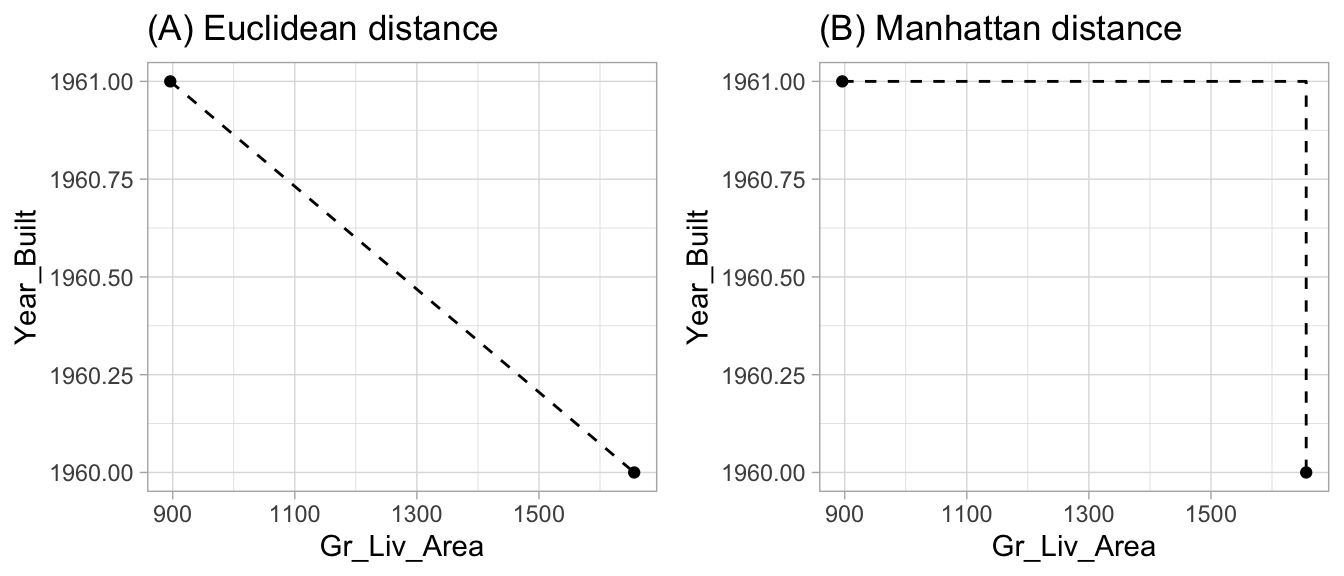

Figure 8.2: Euclidean (A) versus Manhattan (B) distance.

There are other metrics to measure the distance between observations. For example, the Minkowski distance is a generalization of the Euclidean and Manhattan distances and is defined as

\[\begin{equation} \tag{8.3} \bigg( \sum^P_{j=1} | x_{aj} - x_{bj} | ^q \bigg)^{\frac{1}{q}}, \end{equation}\]

where \(q > 0\) (Han, Pei, and Kamber 2011). When \(q = 2\) the Minkowski distance equals the Euclidean distance and when \(q = 1\) it is equal to the Manhattan distance. The Mahalanobis distance is also an attractive measure to use since it accounts for the correlation between two variables (De Maesschalck, Jouan-Rimbaud, and Massart 2000).

8.2.2 Pre-processing

Due to the squaring in Equation (8.1), the Euclidean distance is more sensitive to outliers. Furthermore, most distance measures are sensitive to the scale of the features. Data with features that have different scales will bias the distance measures as those predictors with the largest values will contribute most to the distance between two samples. For example, consider the three home below: home1 is a four bedroom built in 2008, home2 is a two bedroom built in the same year, and home3 is a three bedroom built a decade earlier.

home1
## # A tibble: 1 x 4
##   home  Bedroom_AbvGr Year_Built    id
##   <chr>         <int>      <int> <int>
## 1 home1             4       2008   423
home2
## # A tibble: 1 x 4
##   home  Bedroom_AbvGr Year_Built    id
##   <chr>         <int>      <int> <int>
## 1 home2             2       2008   424
home3
## # A tibble: 1 x 4
##   home  Bedroom_AbvGr Year_Built    id
##   <chr>         <int>      <int> <int>
## 1 home3             3       1998     6

The Euclidean distance between home1 and home3 is larger due to the larger difference in Year_Built with home2.

features <- c("Bedroom_AbvGr", "Year_Built")

# distance between home 1 and 2
dist(rbind(home1[,features], home2[,features]))
##   1
## 2 2

# distance between home 1 and 3
dist(rbind(home1[,features], home3[,features]))
##          1
## 2 10.04988

However, Year_Built has a much larger range (1875–2010) than Bedroom_AbvGr (0–8). And if you ask most people, especially families with kids, the difference between 2 and 4 bedrooms is much more significant than a 10 year difference in the age of a home. If we standardize these features, we see that the difference between home1 and home2’s standardized value for Bedroom_AbvGr is larger than the difference between home1 and home3’s Year_Built. And if we compute the Euclidean distance between these standardized home features, we see that now home1 and home3 are more similar than home1 and home2.

home1_std
## # A tibble: 1 x 4
##   home  Bedroom_AbvGr Year_Built    id
##   <chr>         <dbl>      <dbl> <int>
## 1 home1          1.38       1.21   423
home2_std
## # A tibble: 1 x 4
##   home  Bedroom_AbvGr Year_Built    id
##   <chr>         <dbl>      <dbl> <int>
## 1 home2         -1.03       1.21   424
home3_std
## # A tibble: 1 x 4
##   home  Bedroom_AbvGr Year_Built    id
##   <chr>         <dbl>      <dbl> <int>
## 1 home3         0.176      0.881     6

# distance between home 1 and 2
dist(rbind(home1_std[,features], home2_std[,features]))
##          1
## 2 2.416244

# distance between home 1 and 3
dist(rbind(home1_std[,features], home3_std[,features]))
##          1
## 2 1.252547

In addition to standardizing numeric features, all categorical features must be one-hot encoded or encoded using another method (e.g., ordinal encoding) so that all categorical features are represented numerically. Furthermore, the KNN method is very sensitive to noisy predictors since they cause similar samples to have larger magnitudes and variability in distance values. Consequently, removing irrelevant, noisy features often leads to significant improvement.

8.3 Choosing k

The performance of KNNs is very sensitive to the choice of \(k\). This was illustrated in Section 2.5.3 where low values of \(k\) typically overfit and large values often underfit. At the extremes, when \(k = 1\), we base our prediction on a single observation that has the closest distance measure. In contrast, when \(k = n\), we are simply using the average (regression) or most common class (classification) across all training samples as our predicted value.

There is no general rule about the best \(k\) as it depends greatly on the nature of the data. For high signal data with very few noisy (irrelevant) features, smaller values of \(k\) tend to work best. As more irrelevant features are involved, larger values of \(k\) are required to smooth out the noise. To illustrate, we saw in Section 3.8.3 that we optimized the RMSE for the ames_train data with \(k = 12\). The ames_train data has 2054 observations, so such a small \(k\) likely suggests a strong signal exists. In contrast, the churn_train data has 1030 observations and Figure 8.3 illustrates that our loss function is not optimized until \(k = 271\). Moreover, the max ROC value is 0.8078 and the overall proportion of attriting employees to non-attriting is 0.839. This suggest there is likely not a very strong signal in the Attrition data.

When using KNN for classification, it is best to assess odd numbers for \(k\) to avoid ties in the event there is equal proportion of response levels (i.e. when k = 2 one of the neighbors could have class “0” while the other neighbor has class “1”).

# Create blueprint
blueprint <- recipe(Attrition ~ ., data = churn_train) %>%
  step_nzv(all_nominal()) %>%
  step_integer(contains("Satisfaction")) %>%
  step_integer(WorkLifeBalance) %>%
  step_integer(JobInvolvement) %>%
  step_dummy(all_nominal(), -all_outcomes(), one_hot = TRUE) %>%
  step_center(all_numeric(), -all_outcomes()) %>%
  step_scale(all_numeric(), -all_outcomes())

# Create a resampling method
cv <- trainControl(
  method = "repeatedcv", 
  number = 10, 
  repeats = 5,
  classProbs = TRUE,                 
  summaryFunction = twoClassSummary
)

# Create a hyperparameter grid search
hyper_grid <- expand.grid(
  k = floor(seq(1, nrow(churn_train)/3, length.out = 20))
)

# Fit knn model and perform grid search
knn_grid <- train(
  blueprint, 
  data = churn_train, 
  method = "knn", 
  trControl = cv, 
  tuneGrid = hyper_grid,
  metric = "ROC"
)

ggplot(knn_grid)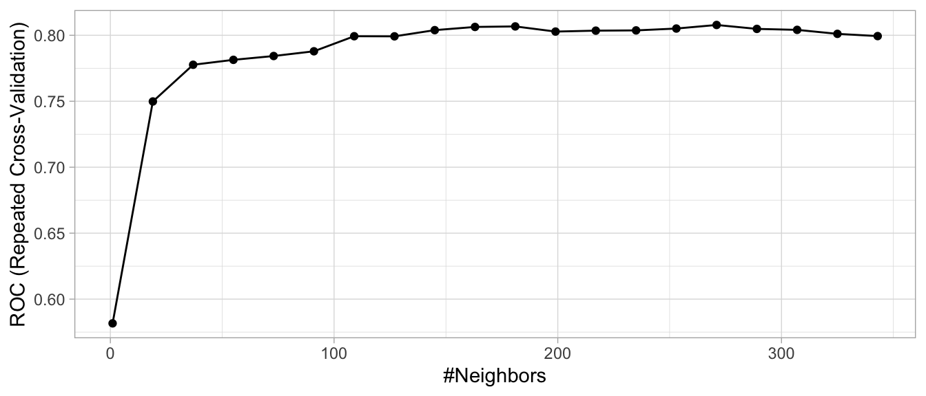

Figure 8.3: Cross validated search grid results for Attrition training data where 20 values between 1 and 343 are assessed for k. When k = 1, the predicted value is based on a single observation that is closest to the target sample and when k = 343, the predicted value is based on the response with the largest proportion for 1/3 of the training sample.

8.4 MNIST example

The MNIST data set is significantly larger than the Ames housing and attrition data sets. Because we want this example to run locally and in a reasonable amount of time (< 1 hour), we will train our initial models on a random sample of 10,000 rows from the training set.

set.seed(123)
index <- sample(nrow(mnist$train$images), size = 10000)
mnist_x <- mnist$train$images[index, ]
mnist_y <- factor(mnist$train$labels[index])

Recall that the MNIST data contains 784 features representing the darkness (0–255) of pixels in images of handwritten numbers (0–9). As stated in Section 8.2.2, KNN models can be severely impacted by irrelevant features. One culprit of this is zero, or near-zero variance features (see Section 3.4). Figure 8.4 illustrates that there are nearly 125 features that have zero variance and many more that have very little variation.

mnist_x %>%
  as.data.frame() %>%
  map_df(sd) %>%
  gather(feature, sd) %>%
  ggplot(aes(sd)) +
  geom_histogram(binwidth = 1)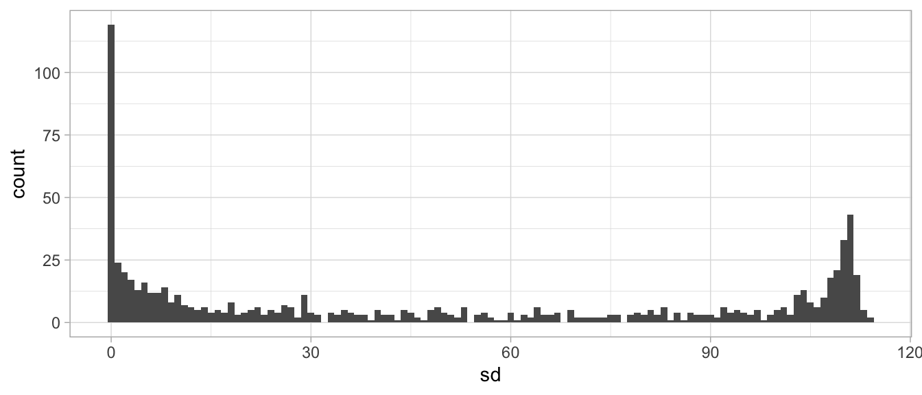

Figure 8.4: Distribution of variability across the MNIST features. We see a significant number of zero variance features that should be removed.

Figure 8.5 shows which features are driving this concern. Images (A)–(C) illustrate typical handwritten numbers from the test set. Image (D) illustrates which features in our images have variability. The white in the center shows that the features that represent the center pixels have regular variability whereas the black exterior highlights that the features representing the edge pixels in our images have zero or near-zero variability. These features have low variability in pixel values because they are rarely drawn on.

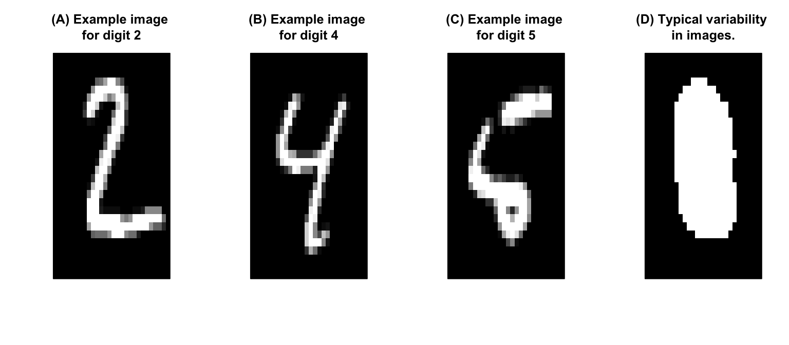
Figure 8.5: Example images (A)-(C) from our data set and (D) highlights near-zero variance features around the edges of our images.

By identifying and removing these zero (or near-zero) variance features, we end up keeping 249 of the original 784 predictors. This can cause dramatic improvements to both the accuracy and speed of our algorithm. Furthermore, by removing these upfront we can remove some of the overhead experienced by caret::train(). Furthermore, we need to add column names to the feature matrices as these are required by caret.

# Rename features
colnames(mnist_x) <- paste0("V", 1:ncol(mnist_x))

# Remove near zero variance features manually
nzv <- nearZeroVar(mnist_x)
index <- setdiff(1:ncol(mnist_x), nzv)
mnist_x <- mnist_x[, index]

Next we perform our search grid. Since we are working with a larger data set, using resampling (e.g., \(k\)-fold cross validation) becomes costly. Moreover, as we have more data, our estimated error rate produced by a simple train vs. validation set becomes less biased and variable. Consequently, the following CV procedure (cv) uses 70% of our data to train and the remaining 30% for validation. We can adjust the number of times we do this which becomes similar to the bootstrap procedure discussed in Section 2.4.

Our hyperparameter grid search assesses 13 \(k\) values between 1–25 and takes approximately 3 minutes.

# Use train/validate resampling method
cv <- trainControl(
  method = "LGOCV", 
  p = 0.7,
  number = 1,
  savePredictions = TRUE
)

# Create a hyperparameter grid search
hyper_grid <- expand.grid(k = seq(3, 25, by = 2))

# Execute grid search
knn_mnist <- train(
  mnist_x,
  mnist_y,
  method = "knn",
  tuneGrid = hyper_grid,
  preProc = c("center", "scale"),
  trControl = cv
)

ggplot(knn_mnist)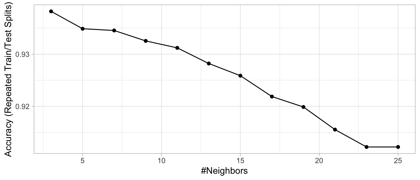

Figure 8.6: KNN search grid results for the MNIST data

Figure 8.6 illustrates the grid search results and our best model used 3 nearest neighbors and provided an accuracy of 93.8%. Looking at the results for each class, we can see that 8s were the hardest to detect followed by 2s, 3s, and 4s (based on sensitivity). The most common incorrectly predicted digit is 1 (specificity).

# Create confusion matrix
cm <- confusionMatrix(knn_mnist$pred$pred, knn_mnist$pred$obs)
cm$byClass[, c(1:2, 11)]  # sensitivity, specificity, & accuracy
##          Sensitivity Specificity Balanced Accuracy
## Class: 0   0.9641638   0.9962374         0.9802006
## Class: 1   0.9916667   0.9841210         0.9878938
## Class: 2   0.9155666   0.9955114         0.9555390
## Class: 3   0.9163952   0.9920325         0.9542139
## Class: 4   0.8698630   0.9960538         0.9329584
## Class: 5   0.9151404   0.9914891         0.9533148
## Class: 6   0.9795322   0.9888684         0.9842003
## Class: 7   0.9326520   0.9896962         0.9611741
## Class: 8   0.8224382   0.9978798         0.9101590
## Class: 9   0.9329897   0.9852687         0.9591292

Feature importance for KNNs is computed by finding the features with the smallest distance measure (see Equation (8.1)). Since the response variable in the MNIST data is multiclass, the variable importance scores below sort the features by maximum importance across the classes.

# Top 20 most important features
vi <- varImp(knn_mnist)
vi
## ROC curve variable importance
## 
##   variables are sorted by maximum importance across the classes
##   only 20 most important variables shown (out of 249)
## 
##          X0     X1     X2     X3     X4     X5     X6     X7     X8    X9
## V435 100.00 100.00 100.00 100.00 100.00 100.00 100.00 100.00 100.00 80.56
## V407  99.42  99.42  99.42  99.42  99.42  99.42  99.42  99.42  99.42 75.21
## V463  97.88  97.88  97.88  97.88  97.88  97.88  97.88  97.88  97.88 83.27
## V379  97.38  97.38  97.38  97.38  97.38  97.38  97.38  97.38  97.38 86.56
## V434  95.87  95.87  95.87  95.87  95.87  95.87  96.66  95.87  95.87 76.20
## V380  96.10  96.10  96.10  96.10  96.10  96.10  96.10  96.10  96.10 88.04
## V462  95.56  95.56  95.56  95.56  95.56  95.56  95.56  95.56  95.56 83.38
## V408  95.37  95.37  95.37  95.37  95.37  95.37  95.37  95.37  95.37 75.05
## V352  93.55  93.55  93.55  93.55  93.55  93.55  93.55  93.55  93.55 87.13
## V490  93.07  93.07  93.07  93.07  93.07  93.07  93.07  93.07  93.07 81.88
## V406  92.90  92.90  92.90  92.90  92.90  92.90  92.90  92.90  92.90 74.55
## V437  70.79  60.44  92.79  52.04  71.11  83.42  75.51  91.15  52.02 70.79
## V351  92.41  92.41  92.41  92.41  92.41  92.41  92.41  92.41  92.41 82.08
## V409  70.55  76.12  88.11  54.54  79.94  77.69  84.88  91.91  52.72 76.12
## V436  89.96  89.96  90.89  89.96  89.96  89.96  91.39  89.96  89.96 78.83
## V464  76.73  76.51  90.24  76.51  76.51  76.58  77.67  82.02  76.51 76.73
## V491  89.49  89.49  89.49  89.49  89.49  89.49  89.49  89.49  89.49 77.41
## V598  68.01  68.01  88.44  68.01  68.01  84.92  68.01  88.25  68.01 38.76
## V465  63.09  36.58  87.68  38.16  50.72  80.62  59.88  84.28  57.13 63.09
## V433  63.74  55.69  76.69  55.69  57.43  55.69  87.59  68.44  55.69 63.74

We can plot these results to get an understanding of what pixel features are driving our results. The image shows that the most influential features lie around the edges of numbers (outer white circle) and along the very center. This makes intuitive sense as many key differences between numbers lie in these areas. For example, the main difference between a 3 and an 8 is whether the left side of the number is enclosed.

# Get median value for feature importance
imp <- vi$importance %>%
  rownames_to_column(var = "feature") %>%
  gather(response, imp, -feature) %>%
  group_by(feature) %>%
  summarize(imp = median(imp))

# Create tibble for all edge pixels
edges <- tibble(
  feature = paste0("V", nzv),
  imp = 0
)

# Combine and plot
imp <- rbind(imp, edges) %>%
  mutate(ID  = as.numeric(str_extract(feature, "\\d+"))) %>%
  arrange(ID)
image(matrix(imp$imp, 28, 28), col = gray(seq(0, 1, 0.05)), 
      xaxt="n", yaxt="n")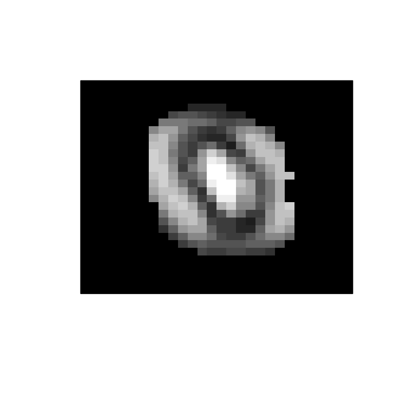

Figure 8.7: Image heat map showing which features, on average, are most influential across all response classes for our KNN model.

We can look at a few of our correct (left) and incorrect (right) predictions in Figure 8.8. When looking at the incorrect predictions, we can rationalize some of the errors (e.g., the actual 4 where we predicted a 1 has a strong vertical stroke compared to the rest of the number’s features, the actual 2 where we predicted a 0 is blurry and not well defined.)

# Get a few accurate predictions
set.seed(9)
good <- knn_mnist$pred %>%
  filter(pred == obs) %>%
  sample_n(4)

# Get a few inaccurate predictions
set.seed(9)
bad <- knn_mnist$pred %>%
  filter(pred != obs) %>%
  sample_n(4)

combine <- bind_rows(good, bad)

# Get original feature set with all pixel features
set.seed(123)
index <- sample(nrow(mnist$train$images), 10000)
X <- mnist$train$images[index,]

# Plot results
par(mfrow = c(4, 2), mar=c(1, 1, 1, 1))
layout(matrix(seq_len(nrow(combine)), 4, 2, byrow = FALSE))
for(i in seq_len(nrow(combine))) {
  image(matrix(X[combine$rowIndex[i],], 28, 28)[, 28:1], 
        col = gray(seq(0, 1, 0.05)),
        main = paste("Actual:", combine$obs[i], "  ", 
                     "Predicted:", combine$pred[i]),
        xaxt="n", yaxt="n") 
}

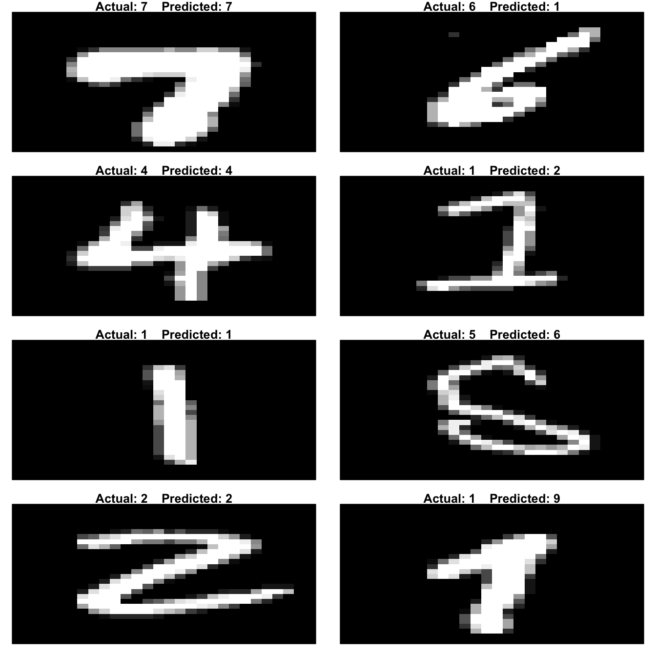
Figure 8.8: Actual images from the MNIST data set along with our KNN model’s predictions. Left column illustrates a few accurate predictions and the right column illustrates a few inaccurate predictions.

8.5 Final thoughts

KNNs are a very simplistic, and intuitive, algorithm that can provide average to decent predictive power, especially when the response is dependent on the local structure of the features. However, a major drawback of KNNs is their computation time, which increases by \(n \times p\) for each observation. Furthermore, since KNNs are a lazy learner, they require the model be run at prediction time which limits their use for real-time modeling. Some work has been done to minimize this effect; for example the FNN package (Beygelzimer et al. 2019) provides a collection of fast \(k\)-nearest neighbor search algorithms and applications such as cover-tree (Beygelzimer, Kakade, and Langford 2006) and kd-tree (Robinson 1981).

Although KNNs rarely provide the best predictive performance, they have many benefits, for example, in feature engineering and in data cleaning and preprocessing. We discussed KNN for imputation in Section 3.3.2. Bruce and Bruce (2017) discuss another approach that uses KNNs to add a local knowledge feature. This includes running a KNN to estimate the predicted output or class and using this predicted value as a new feature for downstream modeling. However, this approach also invites more opportunities for target leakage.

Other alternatives to traditional KNNs such as using invariant metrics, tangent distance metrics, and adaptive nearest neighbor methods are also discussed in J. Friedman, Hastie, and Tibshirani (2001) and are worth exploring.

References

Beygelzimer, Alina, Sham Kakade, and John Langford. 2006. “Cover Trees for Nearest Neighbor.” In Proceedings of the 23rd International Conference on Machine Learning, 97–104. ACM.

Beygelzimer, Alina, Sham Kakadet, John Langford, Sunil Arya, David Mount, and Shengqiao Li. 2019. FNN: Fast Nearest Neighbor Search Algorithms and Applications. https://CRAN.R-project.org/package=FNN.

Bruce, Peter, and Andrew Bruce. 2017. Practical Statistics for Data Scientists: 50 Essential Concepts. O’Reilly Media, Inc.

Cunningham, Padraig, and Sarah Jane Delany. 2007. “K-Nearest Neighbour Classifiers.” Multiple Classifier Systems 34 (8). Springer New York, NY, USA: 1–17.

De Maesschalck, Roy, Delphine Jouan-Rimbaud, and Désiré L Massart. 2000. “The Mahalanobis Distance.” Chemometrics and Intelligent Laboratory Systems 50 (1). Elsevier: 1–18.

Friedman, Jerome, Trevor Hastie, and Robert Tibshirani. 2001. The Elements of Statistical Learning. Vol. 1. Springer Series in Statistics New York, NY, USA:

Han, Jiawei, Jian Pei, and Micheline Kamber. 2011. Data Mining: Concepts and Techniques. Elsevier.

Jiang, Shengyi, Guansong Pang, Meiling Wu, and Limin Kuang. 2012. “An Improved K-Nearest-Neighbor Algorithm for Text Categorization.” Expert Systems with Applications 39 (1). Elsevier: 1503–9.

Mccord, Michael, and M Chuah. 2011. “Spam Detection on Twitter Using Traditional Classifiers.” In International Conference on Autonomic and Trusted Computing, 175–86. Springer.

Robinson, John T. 1981. “The Kdb-Tree: A Search Structure for Large Multidimensional Dynamic Indexes.” In Proceedings of the 1981 Acm Sigmod International Conference on Management of Data, 10–18. ACM.