Chapter 20 K-means Clustering

In PART III of this book we focused on methods for reducing the dimension of our feature space (\(p\)). The remaining chapters concern methods for reducing the dimension of our observation space (\(n\)); these methods are commonly referred to as clustering. K-means clustering is one of the most commonly used clustering algorithms for partitioning observations into a set of \(k\) groups (i.e. \(k\) clusters), where \(k\) is pre-specified by the analyst. k-means, like other clustering algorithms, tries to classify observations into mutually exclusive groups (or clusters), such that observations within the same cluster are as similar as possible (i.e., high intra-class similarity), whereas observations from different clusters are as dissimilar as possible (i.e., low inter-class similarity). In k-means clustering, each cluster is represented by its center (i.e, centroid) which corresponds to the mean of the observation values assigned to the cluster. The procedure used to find these clusters is similar to the k-nearest neighbor (KNN) algorithm discussed in Chapter 8; albeit, without the need to predict an average response value.

20.1 Prerequisites

For this chapter we’ll use the following packages (note that the primary function to perform k-means, kmeans(), is provided in the stats package that comes with your basic R installation):

# Helper packages
library(dplyr)       # for data manipulation
library(ggplot2)     # for data visualization
library(stringr)     # for string functionality

# Modeling packages
library(cluster)     # for general clustering algorithms
library(factoextra)  # for visualizing cluster results

To illustrate k-means concepts we’ll use the mnist and my_basket data sets from previous chapters. We’ll also discuss clustering with mixed data (e.g., data with both numeric and categorical data types) using the Ames housing data later in the chapter.

mnist <- dslabs::read_mnist()

url <- "https://koalaverse.github.io/homlr/data/my_basket.csv"
my_basket <- readr::read_csv(url)

20.2 Distance measures

The classification of observations into groups requires some method for computing the distance or the (dis)similarity between each pair of observations which form a distance or dissimilarity or matrix.

There are many approaches to calculating these distances; the choice of distance measure is a critical step in clustering (as it was with KNN). It defines how the similarity of two observations (\(x_a\) and \(x_b\) for all \(j\) features) is calculated and it will influence the shape and size of the clusters. Recall from Section 8.2.1 that the classical methods for distance measures are the Euclidean and Manhattan distances; however, alternative distance measures exist such as correlation-based distances, which are widely used for gene expression data; the Gower distance measure (discuss later in Section 20.7), which is commonly used for data sets containing categorical and ordinal features; and cosine distance, which is commonly used in the field of text mining. So how do you decide on a particular distance measure? Unfortunately, there is no straightforward answer and several considerations come into play.

Euclidean distance (i.e., straight line distance, or as the crow flies) is very sensitive to outliers; when they exist they can skew the cluster results which gives false confidence in the compactness of the cluster. If your features follow an approximate Gaussian distribution then Euclidean distance is a reasonable measure to use. However, if your features deviate significantly from normality or if you just want to be more robust to existing outliers, then Manhattan, Minkowski, or Gower distances are often better choices.

If you are analyzing unscaled data where observations may have large differences in magnitude but similar behavior then a correlation-based distance is preferred. For example, say you want to cluster customers based on common purchasing characteristics. It is possible for large volume and low volume customers to exhibit similar behaviors; however, due to their purchasing magnitude the scale of the data may skew the clusters if not using a correlation-based distance measure. Figure 20.1 illustrates this phenomenon where observation one and two purchase similar quantities of items; however, observation two and three have nearly perfect correlation in their purchasing behavior. A non-correlation distance measure would group observations one and two together whereas a correlation-based distance measure would group observations two and three together.

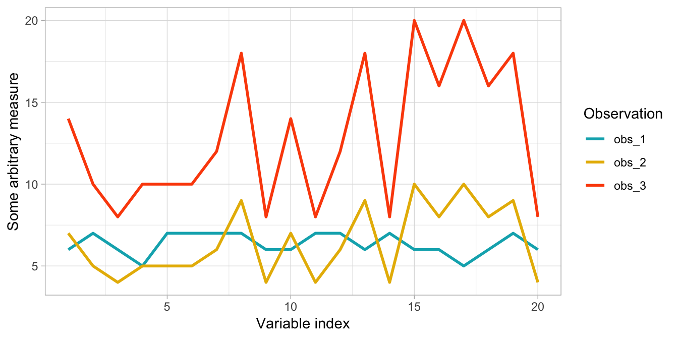
Figure 20.1: Correlation-based distance measures will capture the correlation between two observations better than a non-correlation-based distance measure; regardless of magnitude differences.

20.3 Defining clusters

The basic idea behind k-means clustering is constructing clusters so that the total within-cluster variation is minimized. There are several k-means algorithms available for doing this. The standard algorithm is the Hartigan-Wong algorithm (Hartigan and Wong 1979), which defines the total within-cluster variation as the sum of the Euclidean distances between observation \(i\)’s feature values and the corresponding centroid:

\[\begin{equation} \tag{20.1} W\left(C_k\right) = \sum_{x_i \in C_k}\left(x_{i} - \mu_k\right) ^ 2, \end{equation}\]

where:

• \(x_i\) is an observation belonging to the cluster \(C_k\);
• \(\mu_k\) is the mean value of the points assigned to the cluster \(C_k\).

Each observation (\(x_i\)) is assigned to a given cluster such that the sum of squared (SS) distances of each observation to their assigned cluster centers (\(\mu_k\)) is minimized.

We define the total within-cluster variation as follows:

\[\begin{equation} \tag{20.2} SS_{within} = \sum^k_{k=1}W\left(C_k\right) = \sum^k_{k=1}\sum_{x_i \in C_k}\left(x_i - \mu_k\right)^2 \end{equation}\]

The \(SS_{within}\) measures the compactness (i.e., goodness) of the resulting clusters and we want it to be as small as possible as illustrated in Figure 20.2.

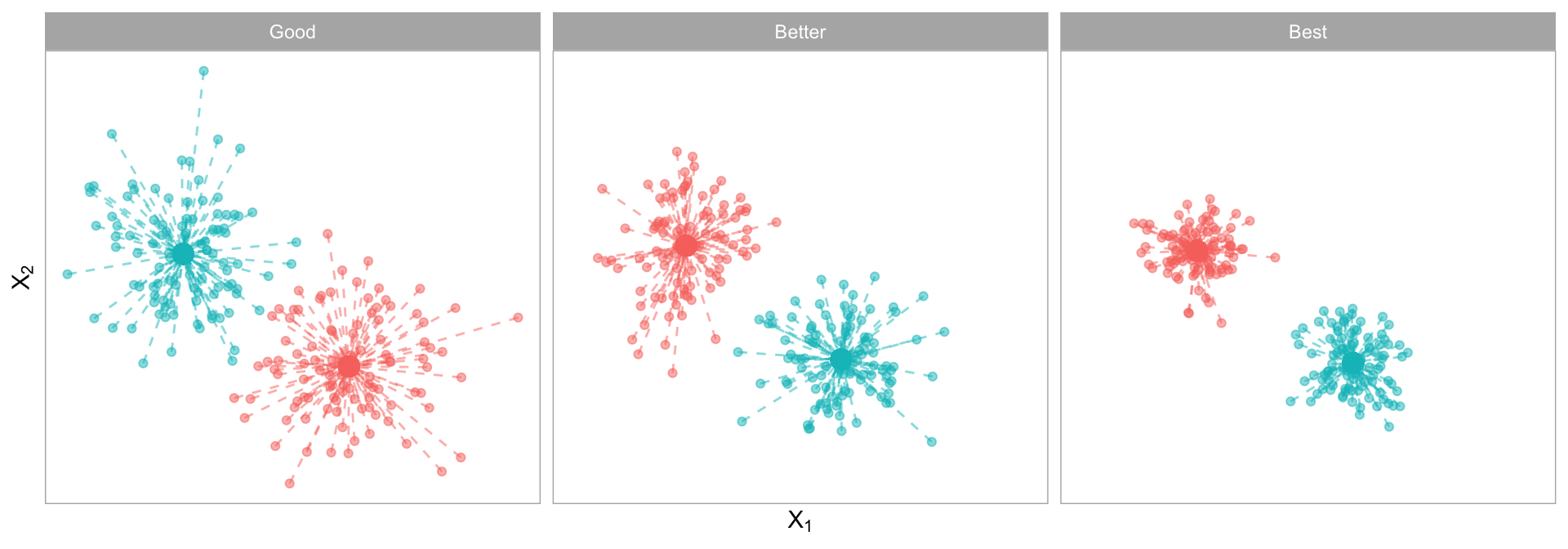
Figure 20.2: Total within-cluster variation captures the total distances between a cluster’s centroid and the individual observations assigned to that cluster. The more compact the these distances, the more defined and isolated the clusters are.

The underlying assumptions of k-means requires points to be closer to their own cluster center than to others. This assumption can be ineffective when the clusters have complicated geometries as k-means requires convex boundaries. For example, consider the data in Figure 20.3 (A). These data are clearly grouped; however, their groupings do not have nice convex boundaries (like the convex boundaries used to illustrate the hard margin classifier in Chapter 14). Consequently, k-means clustering does not capture the appropriate groups as Figure 20.3 (B) illustrates. However, spectral clustering methods apply the same kernal trick discussed in Chapter 14 to allow k-means to discover non-convex boundaries (Figure 20.3 (C)). See J. Friedman, Hastie, and Tibshirani (2001) for a thorough discussion of spectral clustering and the kernlab package for an R implementation. We’ll also discuss model-based clustering methods in Chapter 22 which provide an alternative approach to capture non-convex cluster shapes.

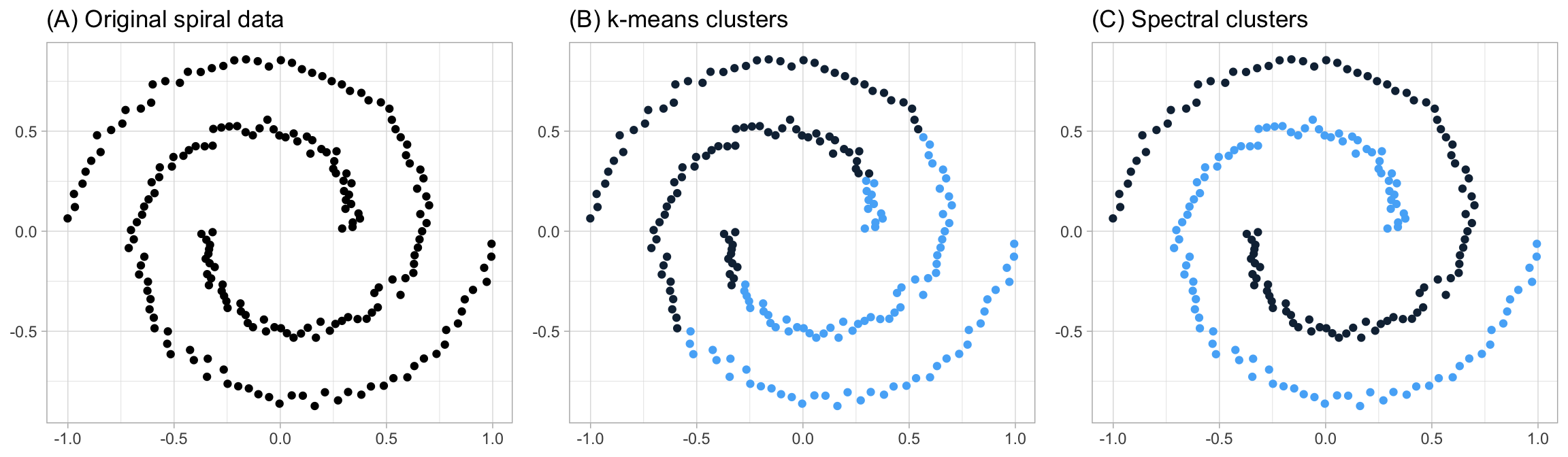
Figure 20.3: The assumptions of k-means lends it ineffective in capturing complex geometric groupings; however, spectral clustering allows you to cluster data that is connected but not necessarily clustered within convex boundaries.

20.4 k-means algorithm

The first step when using k-means clustering is to indicate the number of clusters (\(k\)) that will be generated in the final solution. Unfortunately, unless our data set is very small, we cannot evaluate every possible cluster combination because there are almost \(k^n\) ways to partition \(n\) observations into \(k\) clusters. Consequently, we need to estimate a greedy local optimum solution for our specified \(k\) (Hartigan and Wong 1979). To do so, the algorithm starts by randomly selecting \(k\) observations from the data set to serve as the initial centers for the clusters (i.e., centroids). Next, each of the remaining observations are assigned to its closest centroid, where closest is defined using the distance between the object and the cluster mean (based on the selected distance measure). This is called the cluster assignment step.

Next, the algorithm computes the new center (i.e., mean value) of each cluster. The term centroid update is used to define this step. Now that the centers have been recalculated, every observation is checked again to see if it might be closer to a different cluster. All the objects are reassigned again using the updated cluster means. The cluster assignment and centroid update steps are iteratively repeated until the cluster assignments stop changing (i.e., when convergence is achieved). That is, the clusters formed in the current iteration are the same as those obtained in the previous iteration.

Due to randomization of the initial \(k\) observations used as the starting centroids, we can get slightly different results each time we apply the procedure. Consequently, most algorithms use several random starts and choose the iteration with the lowest \(W\left(C_k\right)\) (Equation (20.1)). Figure 20.4 illustrates the variation in \(W\left(C_k\right)\) for different random starts.

A good rule for the number of random starts to apply is 10–20.

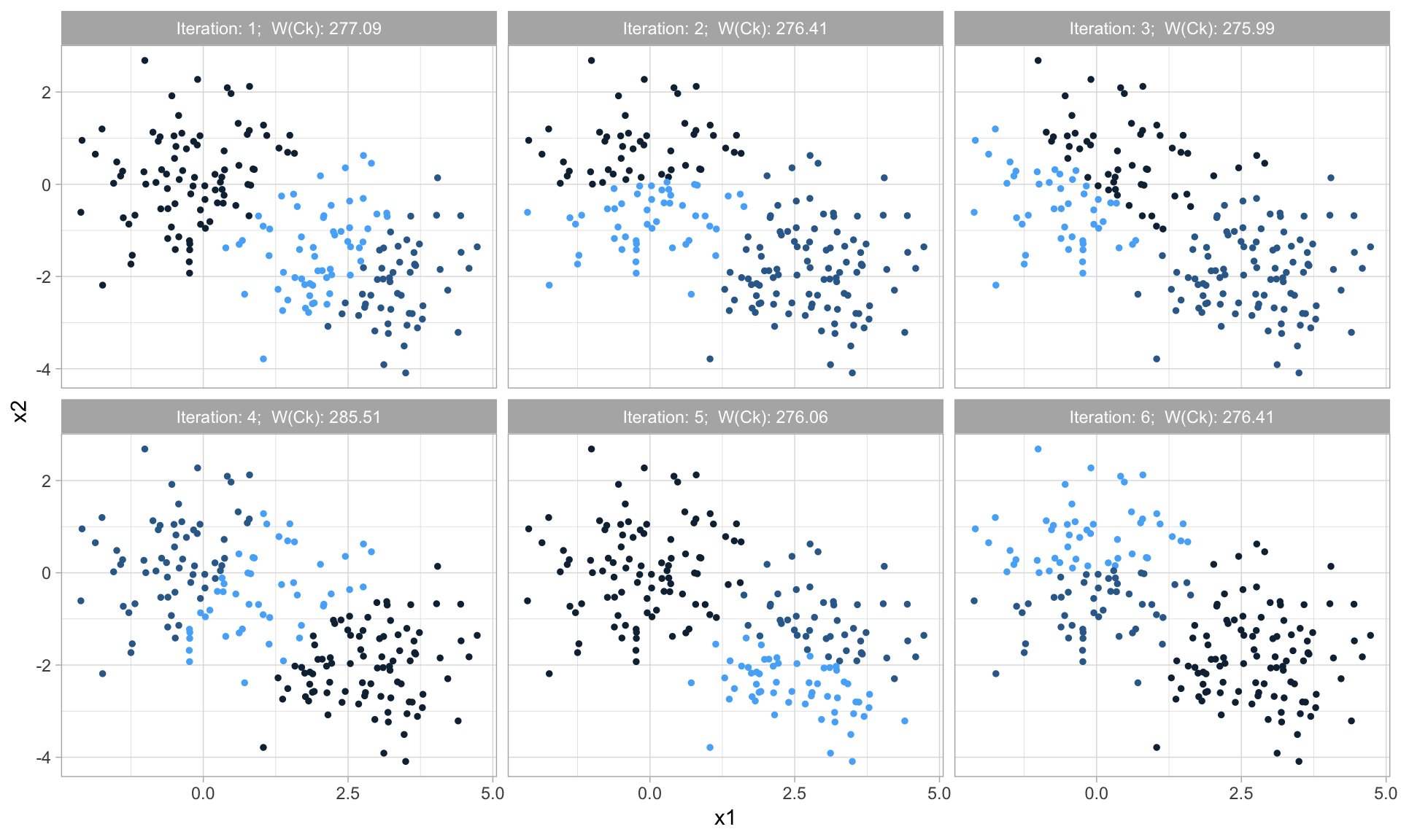
Figure 20.4: Each application of the k-means algorithm can achieve slight differences in the final results based on the random start.

The k-means algorithm can be summarized as follows:

1. Specify the number of clusters (\(k\)) to be created (this is done by the analyst).
2. Select \(k\) observations at random from the data set to use as the initial cluster centroids.
3. Assign each observation to their closest centroid based on the distance measure selected.
4. For each of the \(k\) clusters update the cluster centroid by calculating the new mean values of all the data points in the cluster. The centroid for the \(i\)-th cluster is a vector of length \(p\) containing the means of all \(p\) features for the observations in cluster \(i\).
5. Iteratively minimize \(SS_{within}\). That is, iterate steps 3–4 until the cluster assignments stop changing (beyond some threshold) or the maximum number of iterations is reached. A good rule of thumb is to perform 10–20 iterations.

20.5 Clustering digits

Let’s illustrate an example by performing k-means clustering on the MNIST pixel features and see if we can identify unique clusters of digits without using the response variable. Here, we declare \(k = 10\) only because we already know there are 10 unique digits represented in the data. We also use 10 random starts (nstart = 10). The output of our model contains many of the metrics we’ve already discussed such as total within-cluster variation (withinss), total within-cluster sum of squares (tot.withinss), the size of each cluster (size), and the iteration out of our 10 random starts used (iter). It also includes the cluster each observation is assigned to and the centers of each cluster.

Training k-means on the MNIST data with 10 random starts took about 4.5 minutes for us using the code below.

features <- mnist$train$images

# Use k-means model with 10 centers and 10 random starts
mnist_clustering <- kmeans(features, centers = 10, nstart = 10)

# Print contents of the model output
str(mnist_clustering)
## List of 9
##  $ cluster     : int [1:60000] 5 9 3 8 10 7 4 5 4 6 ...
##  $ centers     : num [1:10, 1:784] 0 0 0 0 0 0 0 0 0 0 ...
##   ..- attr(*, "dimnames")=List of 2
##   .. ..$ : chr [1:10] "1" "2" "3" "4" ...
##   .. ..$ : NULL
##  $ totss       : num 205706725984
##  $ withinss    : num [1:10] 23123576673 14119007546 16438261395 7950166288 ...
##  $ tot.withinss: num 153017742761
##  $ betweenss   : num 52688983223
##  $ size        : int [1:10] 7786 5384 5380 5515 7051 6706 4634 5311 4971 7262
##  $ iter        : int 8
##  $ ifault      : int 0
##  - attr(*, "class")= chr "kmeans"

The centers output is a 10x784 matrix. This matrix contains the average value of each of the 784 features for the 10 clusters. We can plot this as in Figure 20.5 which shows us what the typical digit is in each cluster. We clearly see recognizable digits even though k-means had no insight into the response variable.

# Extract cluster centers
mnist_centers <- mnist_clustering$centers

# Plot typical cluster digits
par(mfrow = c(2, 5), mar=c(0.5, 0.5, 0.5, 0.5))
layout(matrix(seq_len(nrow(mnist_centers)), 2, 5, byrow = FALSE))
for(i in seq_len(nrow(mnist_centers))) {
  image(matrix(mnist_centers[i, ], 28, 28)[, 28:1], 
        col = gray.colors(12, rev = TRUE), xaxt="n", yaxt="n")
}

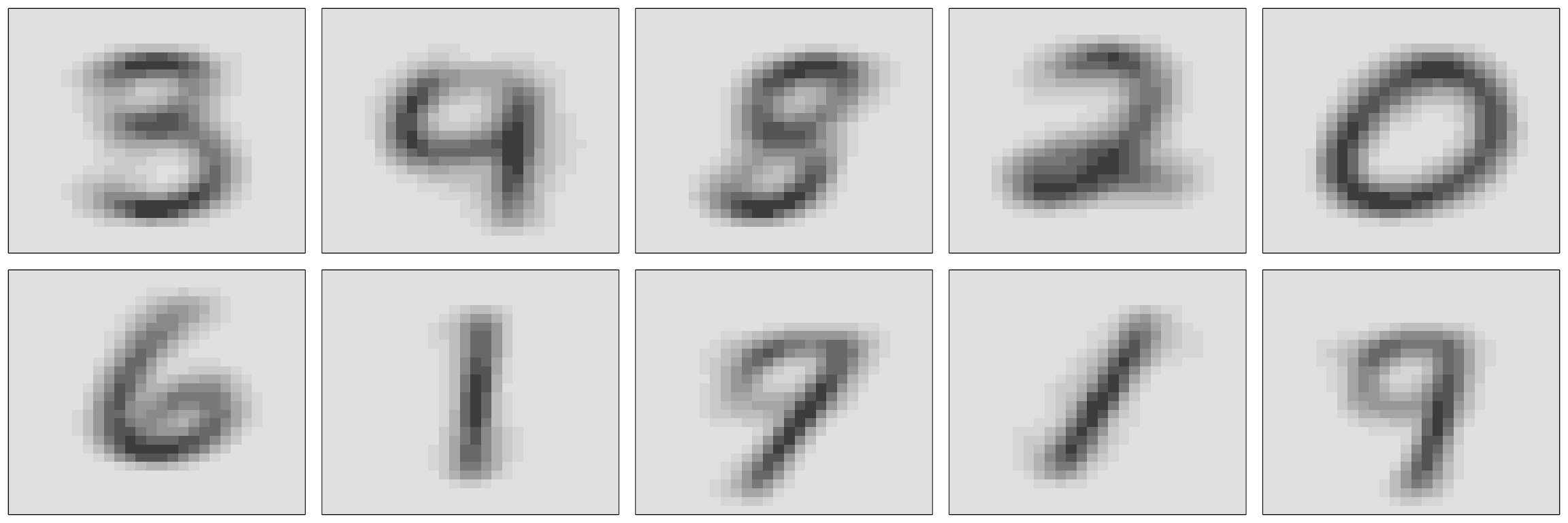
Figure 20.5: Cluster centers for the 10 clusters identified in the MNIST training data.

We can compare the cluster digits with the actual digit labels to see how well our clustering is performing. To do so, we compare the most common digit in each cluster (i.e., with the mode) to the actual training labels. Figure 20.6 illustrates the results. We see that k-means does a decent job of clustering some of the digits. In fact, most of the digits are clustered more often with like digits than with different digits.

However, we also see some digits are grouped often with different digits (e.g., 6s are often grouped with 0s and 9s are often grouped with 7s). We also see that 0s and 5s are never the dominant digit in a cluster. Consequently, our clustering is grouping many digits that have some resemblance (3s, 5s, and 8s are often grouped together) and since this is an unsupervised task, there is no mechanism to supervise the algorithm otherwise.

# Create mode function
mode_fun <- function(x){  
  which.max(tabulate(x))
}

mnist_comparison <- data.frame(
  cluster = mnist_clustering$cluster,
  actual = mnist$train$labels
) %>%
  group_by(cluster) %>%
  mutate(mode = mode_fun(actual)) %>%
  ungroup() %>%
  mutate_all(factor, levels = 0:9)

# Create confusion matrix and plot results
yardstick::conf_mat(
  mnist_comparison, 
  truth = actual, 
  estimate = mode
) %>%
  autoplot(type = 'heatmap')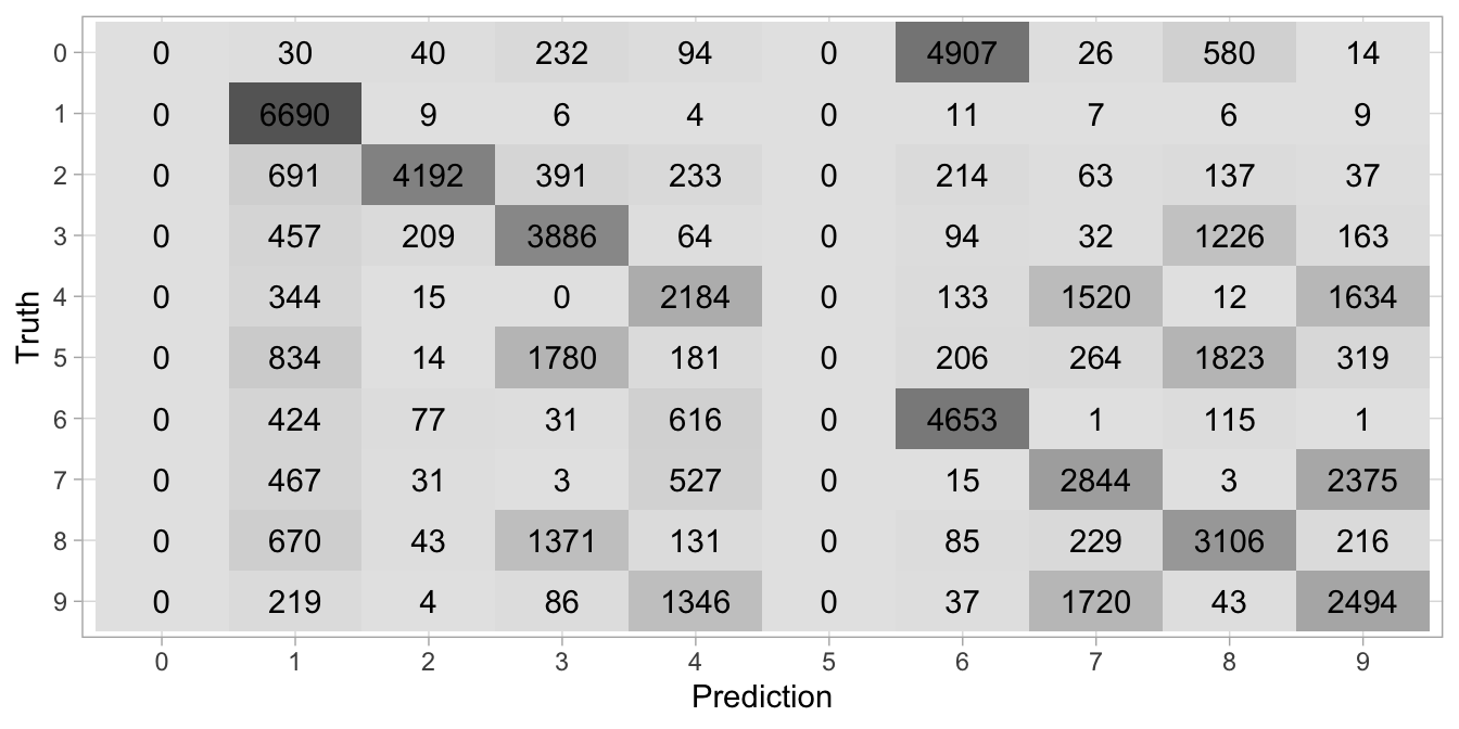

Figure 20.6: Confusion matrix illustrating how the k-means algorithm clustered the digits (x-axis) and the actual labels (y-axis).

20.6 How many clusters?

When clustering the MNIST data, the number of clusters we specified was based on prior knowledge of the data. However, often we do not have this kind of a priori information and the reason we are performing cluster analysis is to identify what clusters may exist. So how do we go about determining the right number of k?

Choosing the number of clusters requires a delicate balance. Larger values of \(k\) can improve homogeneity of the clusters; however it risks overfitting.

Best case (or maybe we should say easiest case) scenario, \(k\) is predetermined. This often occurs when we have deterministic resources to allocate. For example, a company may employ \(k\) sales people and they would like to partition their customers into one of \(k\) segments so that they can be assigned to one of the sales folks. In this case \(k\) is predetermined by external resources or knowledge.

A more common case is that \(k\) is unknown; however, we can often still apply a priori knowledge for potential groupings. For example, maybe you need to cluster customer experience survey responses for an automobile sales company. You may start by setting \(k\) to the number of car brands the company carries. If you lack any a priori knowledge for setting \(k\), then a commonly used rule of thumb is \(k = \sqrt{n/2}\), where \(n\) is the number of observations to cluster. However, this rule can result in very large values of \(k\) for larger data sets (e.g., this would have us use \(k = 173\) for the MNIST data set).

When the goal of the clustering procedure is to ascertain what natural distinct groups exist in the data, without any a priori knowledge, there are multiple statistical methods we can apply. However, many of these measures suffer from the curse of dimensionality as they require multiple iterations and clustering large data sets is not efficient, especially when clustering repeatedly.

See Charrad et al. (2015) for a thorough review of the vast assortment of measures of cluster performance. The NbClust package implements many of these methods, providing you with over 30 indices to determine the optimal \(k\).

One of the more popular methods is the elbow method. Recall that the basic idea behind cluster partitioning methods, such as k-means clustering, is to define clusters such that the total within-cluster variation is minimized (Equation (20.2)). The total within-cluster sum of squares measures the compactness of the clustering and we want it to be as small as possible. Thus, we can use the following approach to define the optimal clusters:

1. Compute k-means clustering for different values of \(k\). For instance, by varying \(k\) from 1–20 clusters.
2. For each \(k\), calculate the total within-cluster sum of squares (WSS).
3. Plot the curve of WSS according to the number of clusters \(k\).
4. The location of a bend (i.e., elbow) in the plot is generally considered as an indicator of the appropriate number of clusters.

When using small to moderate sized data sets this process can be performed conveniently with factoextra::fviz_nbclust(). However, this function requires you to specify a single max \(k\) value and it will train k-means models for \(1-k\) clusters. When dealing with large data sets, such as MNIST, this is unreasonable so you will want to manually implement the procedure (e.g., with a for loop and specify the values of \(k\) to assess).

The following assesses clustering the my_basket data into 1–25 clusters. The method = 'wss' argument specifies that our search criteria is using the elbow method discussed above and since we are assessing quantities across different baskets of goods we use the non-parametric Spearman correlation-based distance measure. The results show the “elbow” appears to happen when \(k = 5\).

fviz_nbclust(
  my_basket, 
  kmeans, 
  k.max = 25,
  method = "wss",
  diss = get_dist(my_basket, method = "spearman")
)

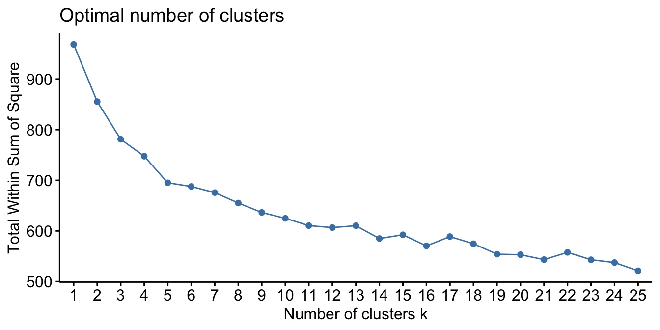
Figure 20.7: Using the elbow method to identify the preferred number of clusters in the my basket data set.

fviz_nbclust() also implements other popular methods such as the Silhouette method (Rousseeuw 1987) and Gap statistic (Tibshirani, Walther, and Hastie 2001). Luckily, applications requiring the exact optimal set of clusters is fairly rare. In most applications, it suffices to choose a \(k\) based on convenience rather than strict performance requirements. But if necessary, the elbow method and other performance metrics can point you in the right direction.

20.7 Clustering with mixed data

Often textbook examples of clustering include only numeric data. However, most real life data sets contain a mixture of numeric, categorical, and ordinal variables; and whether an observation is similar to another observation should depend on these data type attributes. There are a few options for performing clustering with mixed data and we’ll demonstrate on the full Ames housing data set (minus the response variable Sale_Price). To perform k-means clustering on mixed data we can convert any ordinal categorical variables to numeric and one-hot encode the remaining nominal categorical variables.

# Full ames data set --> recode ordinal variables to numeric
ames_full <- AmesHousing::make_ames() %>%
  mutate_if(str_detect(names(.), 'Qual|Cond|QC|Qu'), as.numeric)

# One-hot encode --> retain only the features and not sale price
full_rank  <- caret::dummyVars(Sale_Price ~ ., data = ames_full, 
                               fullRank = TRUE)
ames_1hot <- predict(full_rank, ames_full)

# Scale data
ames_1hot_scaled <- scale(ames_1hot)

# New dimensions
dim(ames_1hot_scaled)
## [1] 2930  240

Now that all our variables are represented numerically, we can perform k-means clustering as we did in the previous sections. Using the elbow method, there does not appear to be a definitive number of clusters to use.

set.seed(123)

fviz_nbclust(
  ames_1hot_scaled, 
  kmeans, 
  method = "wss", 
  k.max = 25, 
  verbose = FALSE
)

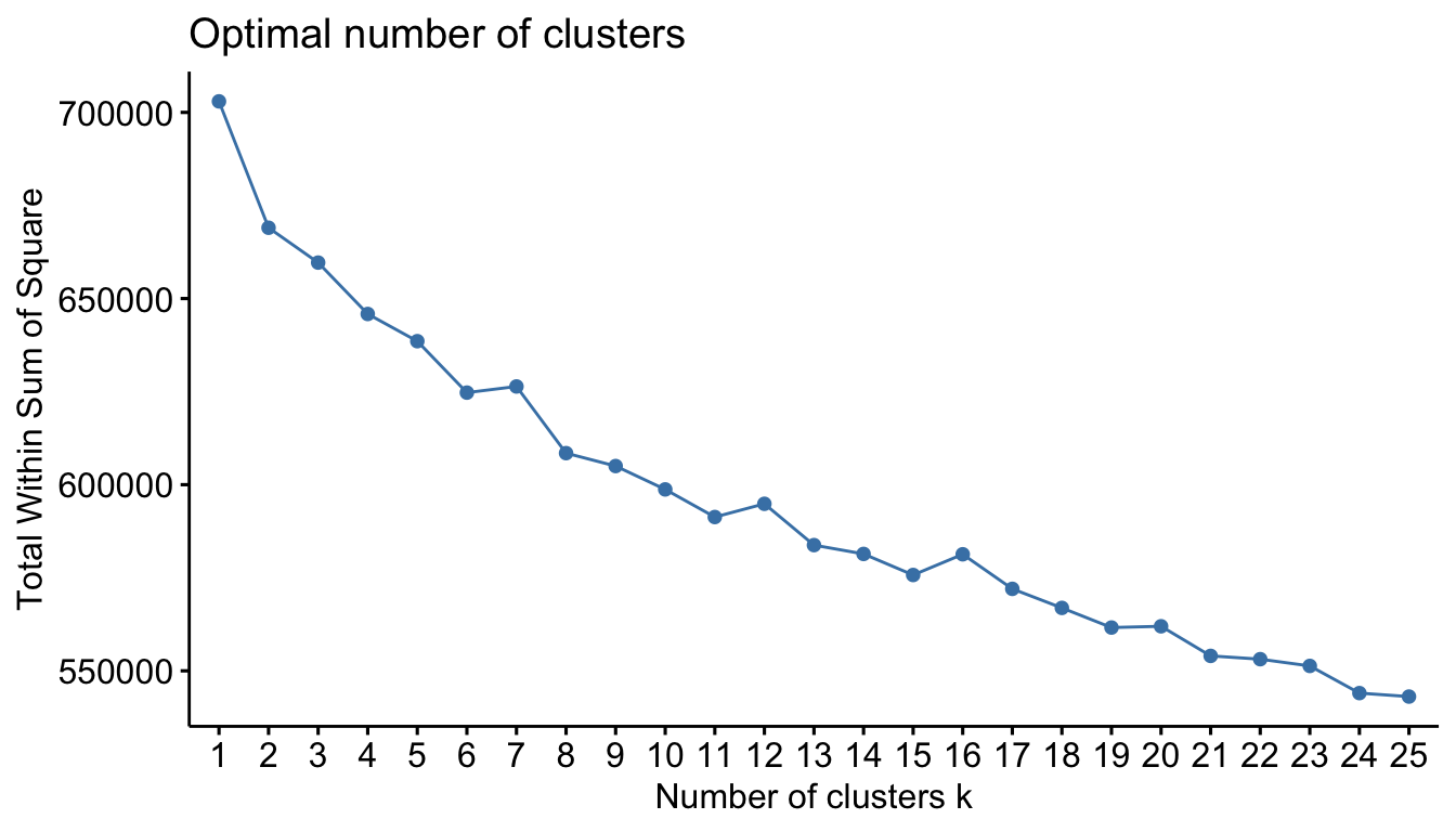
Figure 20.8: Suggested number of clusters for one-hot encoded Ames data using k-means clustering and the elbow criterion.

Unfortunately, this is a common issue. As the number of features expand, performance of k-means tends to break down and both k-means and hierarchical clustering (Chapter 21) approaches become slow and ineffective. This happens, typically, as your data becomes more sparse. An additional option for heavily mixed data is to use the Gower distance (Gower 1971) measure, which applies a particular distance calculation that works well for each data type. The metrics used for each data type include:

• quantitative (interval): range-normalized Manhattan distance;
• ordinal: variable is first ranked, then Manhattan distance is used with a special adjustment for ties;
• nominal: variables with \(k\) categories are first converted into \(k\) binary columns (i.e., one-hot encoded) and then the Dice coefficient is used. To compute the dice metric for two observations \(\left(X, Y\right)\), the algorithm looks across all one-hot encoded categorical variables and scores them as:
  • a — number of dummies 1 for both observations
  • b — number of dummies 1 for \(X\) and 0 for \(Y\)
  • c — number of dummies 0 for \(X\) and 1 for \(Y\)
  • d — number of dummies 0 for both

and then uses the following formula:

\[\begin{equation} \tag{20.3} D = \frac{2a}{2a + b + c} \end{equation}\]

We can use the cluster::daisy() function to create a Gower distance matrix from our data; this function performs the categorical data transformations so you can supply the data in the original format.

# Original data minus Sale_Price
ames_full <- AmesHousing::make_ames() %>% select(-Sale_Price)

# Compute Gower distance for original data
gower_dst <- daisy(ames_full, metric = "gower")

We can now feed the results into any clustering algorithm that accepts a distance matrix. This primarily includes cluster::pam(), cluster::diana(), and cluster::agnes() (stats::kmeans() and cluster::clara() do not accept distance matrices as inputs).

cluster::diana() and cluster::agnes() are hierarchical clustering algorithms that you will learn about in Chapter 21. cluster::pam() and cluster::clara() are discussed in the next section.

# You can supply the Gower distance matrix to several clustering algos
pam_gower <- pam(x = gower_dst, k = 8, diss = TRUE)
diana_gower <- diana(x = gower_dst, diss = TRUE)
agnes_gower <- agnes(x = gower_dst, diss = TRUE)

20.8 Alternative partitioning methods

As your data grow in dimensions you are likely to introduce more outliers; since k-means uses the mean, it is not robust to outliers. An alternative to this is to use partitioning around medians (PAM), which has the same algorithmic steps as k-means but uses the median rather than the mean to determine the centroid; making it more robust to outliers. Unfortunately, this robustness comes with an added computational expense (J. Friedman, Hastie, and Tibshirani 2001).

To perform PAM clustering use cluster::pam() instead of kmeans().

If you compare k-means and PAM clustering results for a given criterion and experience common results then that is a good indication that outliers are not effecting your results. Figure 20.9 illustrates the total within sum of squares for 1–25 clusters using PAM clustering on the one-hot encoded Ames data. We see very similar results as with \(k\)-means (Figure 20.8), which tells us that outliers are not negatively influencing the \(k\)-means results.

fviz_nbclust(
  ames_1hot_scaled, 
  pam, 
  method = "wss", 
  k.max = 25, 
  verbose = FALSE
)

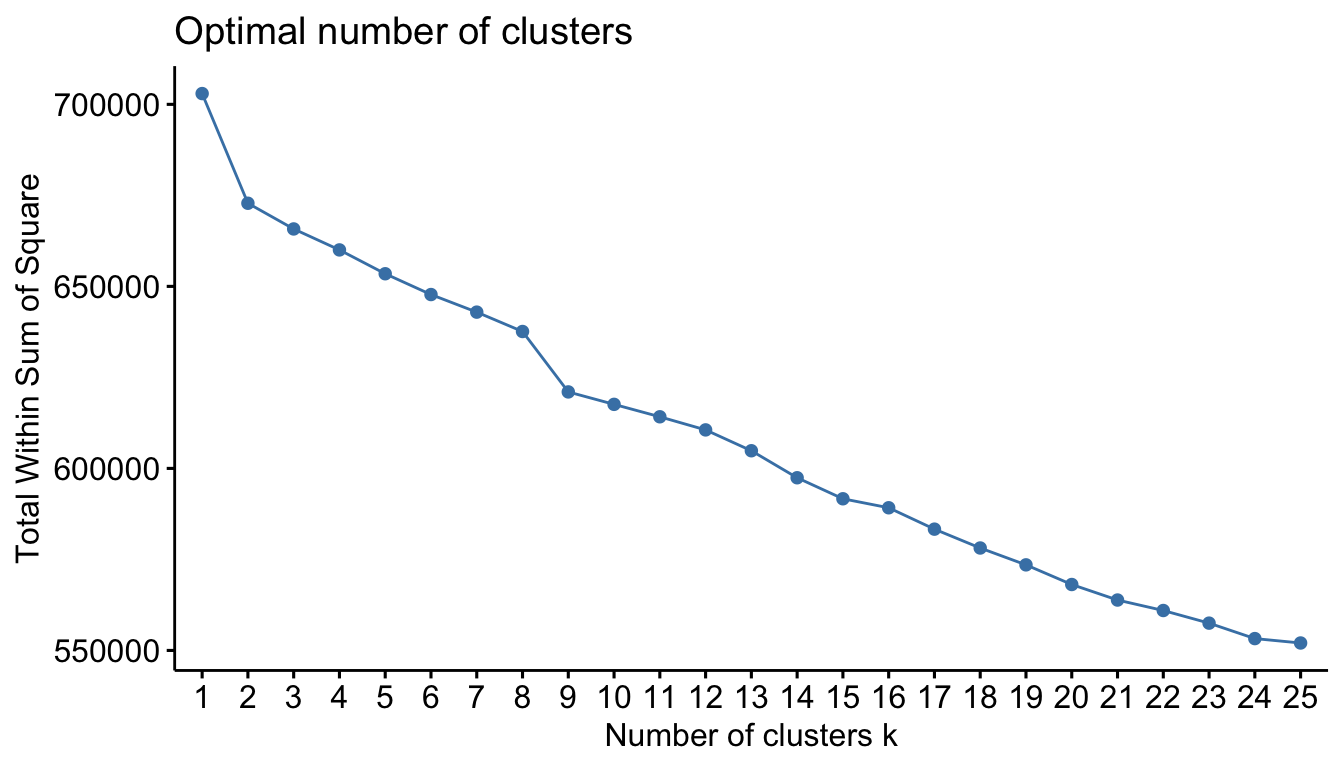
Figure 20.9: Total within sum of squares for 1-25 clusters using PAM clustering.

As your data set becomes larger both hierarchical, k-means, and PAM clustering become slower. An alternative is clustering large applications (CLARA), which performs the same algorithmic process as PAM; however, instead of finding the medoids for the entire data set it considers a small sample size and applies k-means or PAM.

Medoids are similar in spirit to the cluster centers or means, but medoids are always restricted to be members of the data set (similar to the difference between the sample mean and median when you have an odd number of observations and no ties).

CLARA performs the following algorithmic steps:

1. Randomly split the data set into multiple subsets with fixed size.
2. Compute PAM algorithm on each subset and choose the corresponding \(k\) medoids. Assign each observation of the entire data set to the closest medoid.
3. Calculate the mean (or sum) of the dissimilarities of the observations to their closest medoid. This is used as a measure of the goodness of fit of the clustering.
4. Retain the sub-data set for which the mean (or sum) is minimal.

To perform CLARA clustering use cluster::clara() instead of cluster::pam() and kmeans().

If you compute CLARA on the Ames mixed data or on the MNIST data you will find very similar results to both k-means and PAM; however, as the below code illustrates it takes less than \(\frac{1}{5}\)-th of the time!

# k-means computation time on MNIST data
system.time(kmeans(features, centers = 10))
##    user  system elapsed 
## 230.875   4.659 237.404

# CLARA computation time on MNIST data
system.time(clara(features, k = 10))
##   user  system elapsed 
## 37.975   0.286  38.966

20.9 Final thoughts

K-means clustering is probably the most popular clustering algorithm and usually the first applied when solving clustering tasks. Although there have been methods to help analysts identify the optimal number of k clusters, this task is still largely based on subjective inputs and decisions by the analyst considering the unsupervised nature of the algorithm. In the next two chapters we’ll explore alternative approaches that help reduce the burden of the analyst needing to define k. These methods also address other limitations of k-means such as how the algorithm primarily performs well only if the clusters have convex, non-overlapping boundaries; attributes that rarely exists in real data sets.

References

Charrad, Malika, Nadia Ghazzali, Veronique Boiteau, and Azam Niknafs. 2015. NbClust: Determining the Best Number of Clusters in a Data Set. https://CRAN.R-project.org/package=NbClust.

Friedman, Jerome, Trevor Hastie, and Robert Tibshirani. 2001. The Elements of Statistical Learning. Vol. 1. Springer Series in Statistics New York, NY, USA:

Gower, John C. 1971. “A General Coefficient of Similarity and Some of Its Properties.” Biometrics. JSTOR, 857–71.

Hartigan, John A, and Manchek A Wong. 1979. “Algorithm as 136: A K-Means Clustering Algorithm.” Journal of the Royal Statistical Society. Series C (Applied Statistics) 28 (1). JSTOR: 100–108.

Rousseeuw, Peter J. 1987. “Silhouettes: A Graphical Aid to the Interpretation and Validation of Cluster Analysis.” Journal of Computational and Applied Mathematics 20. Elsevier: 53–65.

Tibshirani, Robert, Guenther Walther, and Trevor Hastie. 2001. “Estimating the Number of Clusters in a Data Set via the Gap Statistic.” Journal of the Royal Statistical Society: Series B (Statistical Methodology) 63 (2). Wiley Online Library: 411–23.