Chapter 12 Gradient Boosting
Gradient boosting machines (GBMs) are an extremely popular machine learning algorithm that have proven successful across many domains and is one of the leading methods for winning Kaggle competitions. Whereas random forests (Chapter 11) build an ensemble of deep independent trees, GBMs build an ensemble of shallow trees in sequence with each tree learning and improving on the previous one. Although shallow trees by themselves are rather weak predictive models, they can be “boosted” to produce a powerful “committee” that, when appropriately tuned, is often hard to beat with other algorithms. This chapter will cover the fundamentals to understanding and implementing some popular implementations of GBMs.
12.1 Prerequisites
This chapter leverages the following packages. Some of these packages play a supporting role; however, our focus is on demonstrating how to implement GBMs with the gbm (B Greenwell et al. 2018), xgboost (Chen et al. 2018), and h2o packages.
# Helper packages
library(dplyr)    # for general data wrangling needs

# Modeling packages
library(gbm)      # for original implementation of regular and stochastic GBMs
library(h2o)      # for a java-based implementation of GBM variants
library(xgboost)  # for fitting extreme gradient boosting
We’ll continue working with the ames_train data set created in Section 2.7 to illustrate the main concepts. We’ll also demonstrate h2o functionality using the same setup from Section 11.5.
h2o.init(max_mem_size = "10g")

train_h2o <- as.h2o(ames_train)
response <- "Sale_Price"
predictors <- setdiff(colnames(ames_train), response)
12.2 How boosting works
Several supervised machine learning algorithms are based on a single predictive model, for example: ordinary linear regression, penalized regression models, single decision trees, and support vector machines. Bagging and random forests, on the other hand, work by combining multiple models together into an overall ensemble. New predictions are made by combining the predictions from the individual base models that make up the ensemble (e.g., by averaging in regression). Since averaging reduces variance, bagging (and hence, random forests) are most effectively applied to models with low bias and high variance (e.g., an overgrown decision tree). While boosting is a general algorithm for building an ensemble out of simpler models (typically decision trees), it is more effectively applied to models with high bias and low variance! Although boosting, like bagging, can be applied to any type of model, it is often most effectively applied to decision trees (which we’ll assume from this point on).
12.2.1 A sequential ensemble approach
The main idea of boosting is to add new models to the ensemble sequentially. In essence, boosting attacks the bias-variance-tradeoff by starting with a weak model (e.g., a decision tree with only a few splits) and sequentially boosts its performance by continuing to build new trees, where each new tree in the sequence tries to fix up where the previous one made the biggest mistakes (i.e., each new tree in the sequence will focus on the training rows where the previous tree had the largest prediction errors); see Figure 12.1.
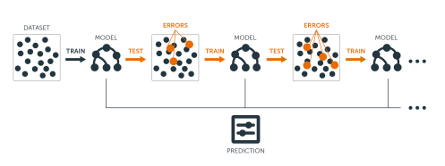
Figure 12.1: Sequential ensemble approach.
Let’s discuss the important components of boosting in closer detail.
The base learners: Boosting is a framework that iteratively improves any weak learning model. Many gradient boosting applications allow you to “plug in” various classes of weak learners at your disposal. In practice however, boosted algorithms almost always use decision trees as the base-learner. Consequently, this chapter will discuss boosting in the context of decision trees.
Training weak models: A weak model is one whose error rate is only slightly better than random guessing. The idea behind boosting is that each model in the sequence slightly improves upon the performance of the previous one (essentially, by focusing on the rows of the training data where the previous tree had the largest errors or residuals). With regards to decision trees, shallow trees (i.e., trees with relatively few splits) represent a weak learner. In boosting, trees with 1–6 splits are most common.
Sequential training with respect to errors: Boosted trees are grown sequentially; each tree is grown using information from previously grown trees to improve performance. This is illustrated in the following algorithm for boosting regression trees. By fitting each tree in the sequence to the previous tree’s residuals, we’re allowing each new tree in the sequence to focus on the previous tree’s mistakes:
- Fit a decision tree to the data: \(F_1\left(x\right) = y\),
- We then fit the next decision tree to the residuals of the previous: \(h_1\left(x\right) = y - F_1\left(x\right)\),
- Add this new tree to our algorithm: \(F_2\left(x\right) = F_1\left(x\right) + h_1\left(x\right)\),
- Fit the next decision tree to the residuals of \(F_2\): \(h_2\left(x\right) = y - F_2\left(x\right)\),
- Add this new tree to our algorithm: \(F_3\left(x\right) = F_2\left(x\right) + h_2\left(x\right)\),
- Continue this process until some mechanism (i.e. cross validation) tells us to stop.
The final model here is a stagewise additive model of b individual trees:
\[ f\left(x\right) = \sum^B_{b=1}f^b\left(x\right) \tag{1} \]
Figure 12.2 illustrates with a simple example where a single predictor (\(x\)) has a true underlying sine wave relationship (blue line) with y along with some irreducible error. The first tree fit in the series is a single decision stump (i.e., a tree with a single split). Each successive decision stump thereafter is fit to the previous one’s residuals. Initially there are large errors, but each additional decision stump in the sequence makes a small improvement in different areas across the feature space where errors still remain.
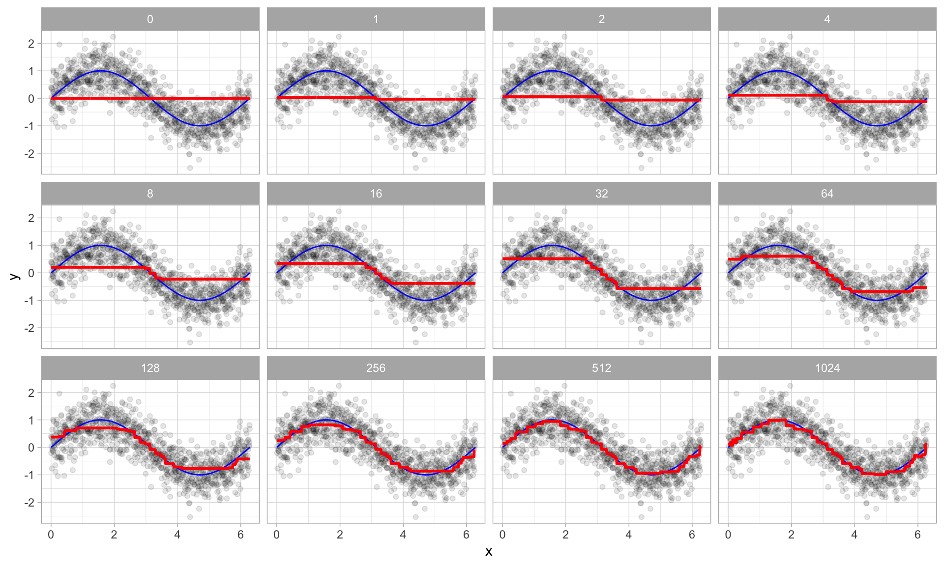
Figure 12.2: Boosted regression decision stumps as 0-1024 successive trees are added.
12.2.2 Gradient descent
Many algorithms in regression, including decision trees, focus on minimizing some function of the residuals; most typically the SSE loss function, or equivalently, the MSE or RMSE (this is accomplished through simple calculus and is the approach taken with least squares). The boosting algorithm for regression discussed in the previous section outlines the approach of sequentially fitting regression trees to the residuals from the previous tree. This specific approach is how gradient boosting minimizes the mean squared error (SSE) loss function (for SSE loss, the gradient is nothing more than the residual error). However, we often wish to focus on other loss functions such as mean absolute error (MAE)—which is less sensitive to outliers—or to be able to apply the method to a classification problem with a loss function such as deviance, or log loss. The name gradient boosting machine comes from the fact that this procedure can be generalized to loss functions other than SSE.
Gradient boosting is considered a gradient descent algorithm. Gradient descent is a very generic optimization algorithm capable of finding optimal solutions to a wide range of problems. The general idea of gradient descent is to tweak parameter(s) iteratively in order to minimize a cost function. Suppose you are a downhill skier racing your friend. A good strategy to beat your friend to the bottom is to take the path with the steepest slope. This is exactly what gradient descent does—it measures the local gradient of the loss (cost) function for a given set of parameters (\(\Theta\)) and takes steps in the direction of the descending gradient. As Figure 12.332 illustrates, once the gradient is zero, we have reached a minimum.
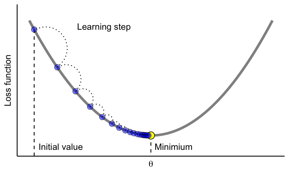
Figure 12.3: Gradient descent is the process of gradually decreasing the cost function (i.e. MSE) by tweaking parameter(s) iteratively until you have reached a minimum.
Gradient descent can be performed on any loss function that is differentiable. Consequently, this allows GBMs to optimize different loss functions as desired (see J. Friedman, Hastie, and Tibshirani (2001), p. 360 for common loss functions). An important parameter in gradient descent is the size of the steps which is controlled by the learning rate. If the learning rate is too small, then the algorithm will take many iterations (steps) to find the minimum. On the other hand, if the learning rate is too high, you might jump across the minimum and end up further away than when you started.
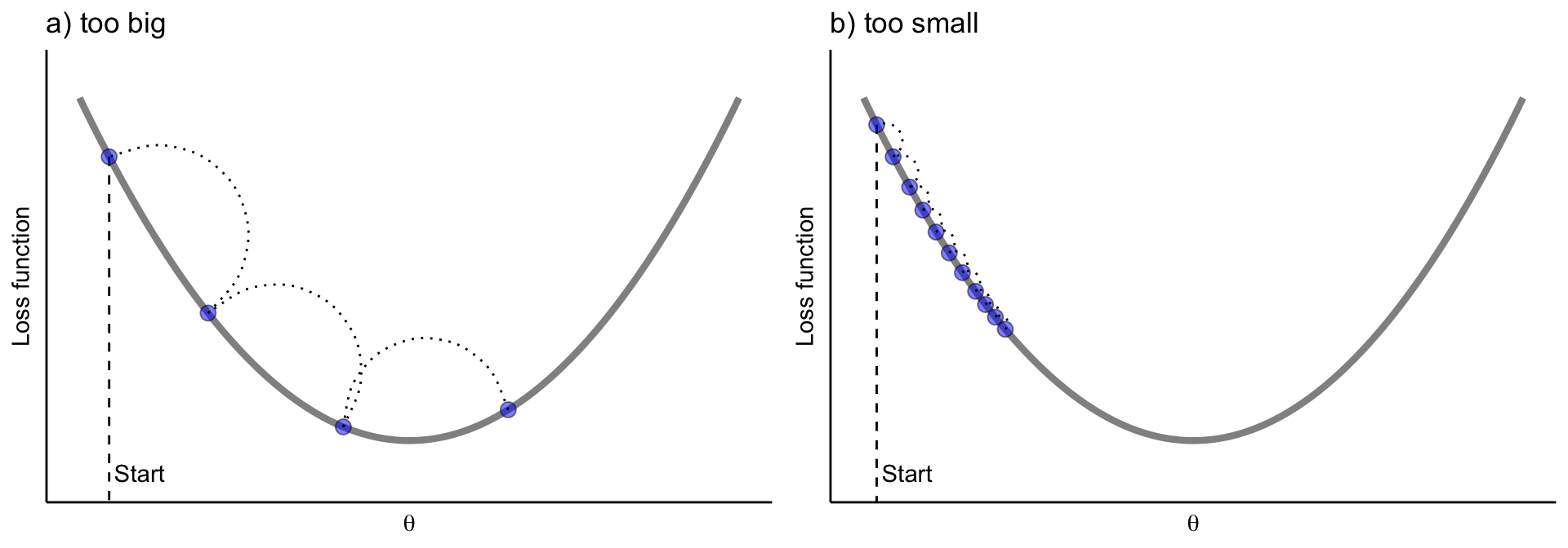
Figure 12.4: A learning rate that is too small will require many iterations to find the minimum. A learning rate too big may jump over the minimum.
Moreover, not all cost functions are convex (i.e., bowl shaped). There may be local minimas, plateaus, and other irregular terrain of the loss function that makes finding the global minimum difficult. Stochastic gradient descent can help us address this problem by sampling a fraction of the training observations (typically without replacement) and growing the next tree using that subsample. This makes the algorithm faster but the stochastic nature of random sampling also adds some random nature in descending the loss function’s gradient. Although this randomness does not allow the algorithm to find the absolute global minimum, it can actually help the algorithm jump out of local minima and off plateaus to get sufficiently near the global minimum.
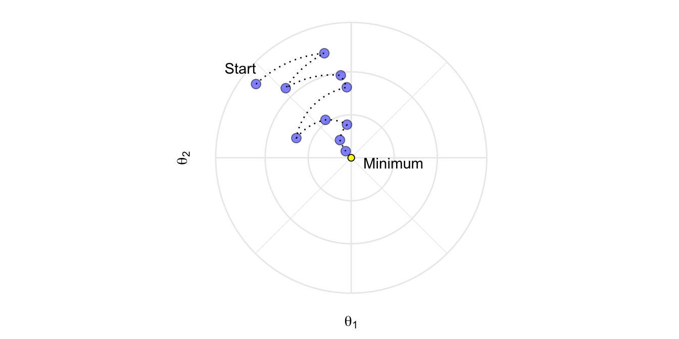
Figure 12.5: Stochastic gradient descent will often find a near-optimal solution by jumping out of local minimas and off plateaus.
As we’ll see in the sections that follow, there are several hyperparameter tuning options available in stochastic gradient boosting (some control the gradient descent and others control the tree growing process). If properly tuned (e.g., with k-fold CV) GBMs can lead to some of the most flexible and accurate predictive models you can build!
12.3 Basic GBM
There are multiple variants of boosting algorithms with the original focused on classification problems (Kuhn and Johnson 2013). Throughout the 1990’s many approaches were developed with the most successful being the AdaBoost algorithm (Freund and Schapire 1999). In 2000, Friedman related AdaBoost to important statistical concepts (e.g., loss functions and additive modeling), which allowed him to generalize the boosting framework to regression problems and multiple loss functions (J. H. Friedman 2001). This led to the typical GBM model that we think of today and that most modern implementations are built on.
12.3.1 Hyperparameters
A simple GBM model contains two categories of hyperparameters: boosting hyperparameters and tree-specific hyperparameters. The two main boosting hyperparameters include:
- Number of trees: The total number of trees in the sequence or ensemble. The averaging of independently grown trees in bagging and random forests makes it very difficult to overfit with too many trees. However, GBMs function differently as each tree is grown in sequence to fix up the past tree’s mistakes. For example, in regression, GBMs will chase residuals as long as you allow them to. Also, depending on the values of the other hyperparameters, GBMs often require many trees (it is not uncommon to have many thousands of trees) but since they can easily overfit we must find the optimal number of trees that minimize the loss function of interest with cross validation.
- Learning rate: Determines the contribution of each tree on the final outcome and controls how quickly the algorithm proceeds down the gradient descent (learns); see Figure 12.3. Values range from 0–1 with typical values between 0.001–0.3. Smaller values make the model robust to the specific characteristics of each individual tree, thus allowing it to generalize well. Smaller values also make it easier to stop prior to overfitting; however, they increase the risk of not reaching the optimum with a fixed number of trees and are more computationally demanding. This hyperparameter is also called shrinkage. Generally, the smaller this value, the more accurate the model can be but also will require more trees in the sequence.
The two main tree hyperparameters in a simple GBM model include:
- Tree depth: Controls the depth of the individual trees. Typical values range from a depth of 3–8 but it is not uncommon to see a tree depth of 1 (J. Friedman, Hastie, and Tibshirani 2001). Smaller depth trees such as decision stumps are computationally efficient (but require more trees); however, higher depth trees allow the algorithm to capture unique interactions but also increase the risk of over-fitting. Note that larger \(n\) or \(p\) training data sets are more tolerable to deeper trees.
- Minimum number of observations in terminal nodes: Also, controls the complexity of each tree. Since we tend to use shorter trees this rarely has a large impact on performance. Typical values range from 5–15 where higher values help prevent a model from learning relationships which might be highly specific to the particular sample selected for a tree (overfitting) but smaller values can help with imbalanced target classes in classification problems.
12.3.2 Implementation
There are many packages that implement GBMs and GBM variants. You can find a fairly comprehensive list at the CRAN Machine Learning Task View: https://cran.r-project.org/web/views/MachineLearning.html. However, the most popular original R implementation of Friedman’s GBM algorithm (J. H. Friedman 2001; Friedman 2002) is the gbm package.
gbm has two training functions: gbm::gbm() and gbm::gbm.fit(). The primary difference is that gbm::gbm() uses the formula interface to specify your model whereas gbm::gbm.fit() requires the separated x and y matrices; gbm::gbm.fit() is more efficient and recommended for advanced users.
The default settings in gbm include a learning rate (shrinkage) of 0.001. This is a very small learning rate and typically requires a large number of trees to sufficiently minimize the loss function. However, gbm uses a default number of trees of 100, which is rarely sufficient. Consequently, we start with a learning rate of 0.1 and increase the number of trees to train. The default depth of each tree (interaction.depth) is 1, which means we are ensembling a bunch of decision stumps (i.e., we are not able to capture any interaction effects). For the Ames housing data set, we increase the tree depth to 3 and use the default value for minimum number of observations required in the trees terminal nodes (n.minobsinnode). Lastly, we set cv.folds = 10 to perform a 10-fold CV.
This model takes a little over 2 minutes to run.
# run a basic GBM model
set.seed(123)  # for reproducibility
ames_gbm1 <- gbm(
  formula = Sale_Price ~ .,
  data = ames_train,
  distribution = "gaussian",  # SSE loss function
  n.trees = 5000,
  shrinkage = 0.1,
  interaction.depth = 3,
  n.minobsinnode = 10,
  cv.folds = 10
)

# find index for number trees with minimum CV error
best <- which.min(ames_gbm1$cv.error)

# get MSE and compute RMSE
sqrt(ames_gbm1$cv.error[best])
## [1] 23240.38
Our results show a cross-validated SSE of 23240 which was achieved with 1219 trees.
# plot error curve
gbm.perf(ames_gbm1, method = "cv")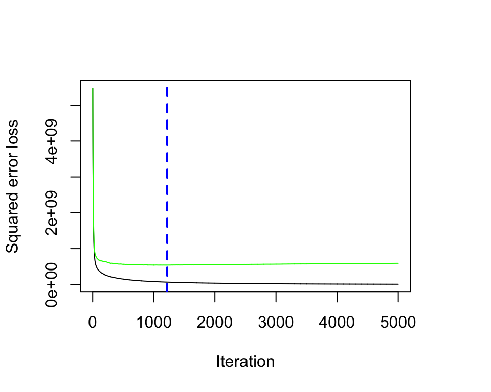
Figure 12.6: Training and cross-validated MSE as n trees are added to the GBM algorithm.
## [1] 121912.3.3 General tuning strategy
Unlike random forests, GBMs can have high variability in accuracy dependent on their hyperparameter settings (Probst, Bischl, and Boulesteix 2018). So tuning can require much more strategy than a random forest model. Often, a good approach is to:
- Choose a relatively high learning rate. Generally the default value of 0.1 works but somewhere between 0.05–0.2 should work across a wide range of problems.
- Determine the optimum number of trees for this learning rate.
- Fix tree hyperparameters and tune learning rate and assess speed vs. performance.
- Tune tree-specific parameters for decided learning rate.
- Once tree-specific parameters have been found, lower the learning rate to assess for any improvements in accuracy.
- Use final hyperparameter settings and increase CV procedures to get more robust estimates. Often, the above steps are performed with a simple validation procedure or 5-fold CV due to computational constraints. If you used k-fold CV throughout steps 1–5 then this step is not necessary.
We already did (1)–(2) in the Ames example above with our first GBM model. Next, we’ll do (3) and asses the performance of various learning rate values between 0.005–0.3. Our results indicate that a learning rate of 0.05 sufficiently minimizes our loss function and requires 2375 trees. All our models take a little over 2 minutes to train so we don’t see any significant impacts in training time based on the learning rate.
The following grid search took us about 10 minutes.
# create grid search
hyper_grid <- expand.grid(
  learning_rate = c(0.3, 0.1, 0.05, 0.01, 0.005),
  RMSE = NA,
  trees = NA,
  time = NA
)

# execute grid search
for(i in seq_len(nrow(hyper_grid))) {

  # fit gbm
  set.seed(123)  # for reproducibility
  train_time <- system.time({
    m <- gbm(
      formula = Sale_Price ~ .,
      data = ames_train,
      distribution = "gaussian",
      n.trees = 5000,
      shrinkage = hyper_grid$learning_rate[i],
      interaction.depth = 3,
      n.minobsinnode = 10,
      cv.folds = 10
   )
  })

  # add SSE, trees, and training time to results
  hyper_grid$RMSE[i]  <- sqrt(min(m$cv.error))
  hyper_grid$trees[i] <- which.min(m$cv.error)
  hyper_grid$Time[i]  <- train_time[["elapsed"]]

}

# results
arrange(hyper_grid, RMSE)
##   learning_rate  RMSE trees  time
## 1         0.050 21382  2375 129.5
## 2         0.010 21828  4982 126.0
## 3         0.100 22252   874 137.6
## 4         0.005 23136  5000 136.8
## 5         0.300 24454   427 139.9
Next, we’ll set our learning rate at the optimal level (0.05) and tune the tree specific hyperparameters (interaction.depth and n.minobsinnode). Adjusting the tree-specific parameters provides us with an additional 600 reduction in RMSE.
This grid search takes about 30 minutes.
# search grid
hyper_grid <- expand.grid(
  n.trees = 6000,
  shrinkage = 0.01,
  interaction.depth = c(3, 5, 7),
  n.minobsinnode = c(5, 10, 15)
)

# create model fit function
model_fit <- function(n.trees, shrinkage, interaction.depth, n.minobsinnode) {
  set.seed(123)
  m <- gbm(
    formula = Sale_Price ~ .,
    data = ames_train,
    distribution = "gaussian",
    n.trees = n.trees,
    shrinkage = shrinkage,
    interaction.depth = interaction.depth,
    n.minobsinnode = n.minobsinnode,
    cv.folds = 10
  )
  # compute RMSE
  sqrt(min(m$cv.error))
}

# perform search grid with functional programming
hyper_grid$rmse <- purrr::pmap_dbl(
  hyper_grid,
  ~ model_fit(
    n.trees = ..1,
    shrinkage = ..2,
    interaction.depth = ..3,
    n.minobsinnode = ..4
    )
)

# results
arrange(hyper_grid, rmse)
##   n.trees shrinkage interaction.depth n.minobsinnode  rmse
## 1    4000      0.05                 5              5 20699
## 2    4000      0.05                 3              5 20723
## 3    4000      0.05                 7              5 21021
## 4    4000      0.05                 3             10 21382
## 5    4000      0.05                 5             10 21915
## 6    4000      0.05                 5             15 21924
## 7    4000      0.05                 3             15 21943
## 8    4000      0.05                 7             10 21999
## 9    4000      0.05                 7             15 22348
After this procedure, we took our top model’s hyperparameter settings, reduced the learning rate to 0.005, and increased the number of trees (8000) to see if we got any additional improvement in accuracy. We experienced no improvement in our RMSE and our training time increased to nearly 6 minutes.
12.4 Stochastic GBMs
An important insight made by Breiman (Breiman (1996a); Breiman (2001)) in developing his bagging and random forest algorithms was that training the algorithm on a random subsample of the training data set offered additional reduction in tree correlation and, therefore, improvement in prediction accuracy. Friedman (2002) used this same logic and updated the boosting algorithm accordingly. This procedure is known as stochastic gradient boosting and, as illustrated in Figure 12.5, helps reduce the chances of getting stuck in local minimas, plateaus, and other irregular terrain of the loss function so that we may find a near global optimum.
12.4.1 Stochastic hyperparameters
There are a few variants of stochastic gradient boosting that can be used, all of which have additional hyperparameters:
- Subsample rows before creating each tree (available in gbm, h2o, & xgboost)
- Subsample columns before creating each tree (h2o & xgboost)
- Subsample columns before considering each split in each tree (h2o & xgboost)
Generally, aggressive subsampling of rows, such as selecting only 50% or less of the training data, has shown to be beneficial and typical values range between 0.5–0.8. Subsampling of columns and the impact to performance largely depends on the nature of the data and if there is strong multicollinearity or a lot of noisy features. Similar to the \(m_{try}\) parameter in random forests (Section 11.4.2), if there are fewer relevant predictors (more noisy data) higher values of column subsampling tends to perform better because it makes it more likely to select those features with the strongest signal. When there are many relevant predictors, a lower values of column subsampling tends to perform well.
When adding in a stochastic procedure, you can either include it in step 4) in the general tuning strategy above (Section 12.3.3), or once you’ve found the optimal basic model (after 6)). In our experience, we have not seen strong interactions between the stochastic hyperparameters and the other boosting and tree-specific hyperparameters.
12.4.2 Implementation
The following uses h2o to implement a stochastic GBM. We use the optimal hyperparameters found in the previous section and build onto this by assessing a range of values for subsampling rows and columns before each tree is built, and subsampling columns before each split. To speed up training we use early stopping for the individual GBM modeling process and also add a stochastic search criteria.
This grid search ran for the entire 60 minutes and evaluated 18 of the possible 27 models.
# refined hyperparameter grid
hyper_grid <- list(
  sample_rate = c(0.5, 0.75, 1),              # row subsampling
  col_sample_rate = c(0.5, 0.75, 1),          # col subsampling for each split
  col_sample_rate_per_tree = c(0.5, 0.75, 1)  # col subsampling for each tree
)

# random grid search strategy
search_criteria <- list(
  strategy = "RandomDiscrete",
  stopping_metric = "mse",
  stopping_tolerance = 0.001,
  stopping_rounds = 10,
  max_runtime_secs = 60*60
)

# perform grid search
grid <- h2o.grid(
  algorithm = "gbm",
  grid_id = "gbm_grid",
  x = predictors,
  y = response,
  training_frame = train_h2o,
  hyper_params = hyper_grid,
  ntrees = 6000,
  learn_rate = 0.01,
  max_depth = 7,
  min_rows = 5,
  nfolds = 10,
  stopping_rounds = 10,
  stopping_tolerance = 0,
  search_criteria = search_criteria,
  seed = 123
)

# collect the results and sort by our model performance metric of choice
grid_perf <- h2o.getGrid(
  grid_id = "gbm_grid",
  sort_by = "mse",
  decreasing = FALSE
)

grid_perf
## H2O Grid Details
## ================
##
## Grid ID: gbm_grid
## Used hyper parameters:
##   -  col_sample_rate
##   -  col_sample_rate_per_tree
##   -  sample_rate
## Number of models: 18
## Number of failed models: 0
##
## Hyper-Parameter Search Summary: ordered by increasing mse
##    col_sample_rate col_sample_rate_per_tree sample_rate         model_ids                  mse
## 1              0.5                      0.5         0.5  gbm_grid_model_8  4.462965966345138E8
## 2              0.5                      1.0         0.5  gbm_grid_model_3  4.568248274796835E8
## 3              0.5                     0.75        0.75 gbm_grid_model_12 4.6466647244785947E8
## 4             0.75                      0.5        0.75  gbm_grid_model_5  4.689665768861389E8
## 5              1.0                     0.75         0.5 gbm_grid_model_14 4.7010349266737276E8
## 6              0.5                      0.5        0.75 gbm_grid_model_10  4.713882927949245E8
## 7             0.75                      1.0         0.5  gbm_grid_model_4  4.729884840420368E8
## 8              1.0                      1.0         0.5  gbm_grid_model_1  4.770705550988762E8
## 9              1.0                     0.75        0.75  gbm_grid_model_6 4.9292332262147874E8
## 10            0.75                      1.0        0.75 gbm_grid_model_13  4.985715082289563E8
## 11            0.75                      0.5         1.0  gbm_grid_model_2 5.0271257831462187E8
## 12            0.75                     0.75        0.75 gbm_grid_model_15 5.0981695262733763E8
## 13            0.75                     0.75         1.0  gbm_grid_model_9 5.3137490858680266E8
## 14            0.75                      1.0         1.0 gbm_grid_model_11   5.77518690995319E8
## 15             1.0                      1.0         1.0  gbm_grid_model_7  6.037512241688542E8
## 16             1.0                     0.75         1.0 gbm_grid_model_16 1.9742225720119803E9
## 17             0.5                      1.0        0.75 gbm_grid_model_17 4.1339991380839005E9
## 18             1.0                      0.5         1.0 gbm_grid_model_18  5.949489361558916E9
Our grid search highlights some important results. Random sampling from the rows for each tree and randomly sampling features before each split appears to positively impact performance. It is not definitive if sampling features before each tree has an impact. Furthermore, the best sampling values are very low (0.5); a further grid search may be beneficial to evaluate even lower values.
The below code chunk extracts the best performing model. In this particular case, we do not see additional improvement in our 10-fold CV RMSE over the best non-stochastic GBM model.
# Grab the model_id for the top model, chosen by cross validation error
best_model_id <- grid_perf@model_ids[[1]]
best_model <- h2o.getModel(best_model_id)

# Now let’s get performance metrics on the best model
h2o.performance(model = best_model, xval = TRUE)
## H2ORegressionMetrics: gbm
## ** Reported on cross-validation data. **
## ** 10-fold cross-validation on training data (Metrics computed for combined holdout predictions) **
##
## MSE:  446296597
## RMSE:  21125.73
## MAE:  13045.95
## RMSLE:  0.1240542
## Mean Residual Deviance :  446296597
12.5 XGBoost
Extreme gradient boosting (XGBoost) is an optimized distributed gradient boosting library that is designed to be efficient, flexible, and portable across multiple languages (Chen and Guestrin 2016). Although XGBoost provides the same boosting and tree-based hyperparameter options illustrated in the previous sections, it also provides a few advantages over traditional boosting such as:
- Regularization: XGBoost offers additional regularization hyperparameters, which we will discuss shortly, that provides added protection against overfitting.
- Early stopping: Similar to h2o, XGBoost implements early stopping so that we can stop model assessment when additional trees offer no improvement.
- Parallel Processing: Since gradient boosting is sequential in nature it is extremely difficult to parallelize. XGBoost has implemented procedures to support GPU and Spark compatibility which allows you to fit gradient boosting using powerful distributed processing engines.
- Loss functions: XGBoost allows users to define and optimize gradient boosting models using custom objective and evaluation criteria.
- Continue with existing model: A user can train an XGBoost model, save the results, and later on return to that model and continue building onto the results. Whether you shut down for the day, wanted to review intermediate results, or came up with additional hyperparameter settings to evaluate, this allows you to continue training your model without starting from scratch.
- Different base learners: Most GBM implementations are built with decision trees but XGBoost also provides boosted generalized linear models.
- Multiple languages: XGBoost offers implementations in R, Python, Julia, Scala, Java, and C++.
In addition to being offered across multiple languages, XGboost can be implemented multiple ways within R. The main R implementation is the xgboost package; however, as illustrated throughout many chapters one can also use caret as a meta engine to implement XGBoost. The h2o package also offers an implementation of XGBoost. In this chapter we’ll demonstrate the xgboost package.
12.5.1 XGBoost hyperparameters
As previously mentioned, xgboost provides the traditional boosting and tree-based hyperparameters we discussed in Sections 12.3.1 and 12.4.1. However, xgboost also provides additional hyperparameters that can help reduce the chances of overfitting, leading to less prediction variability and, therefore, improved accuracy.
12.5.1.1 Regularization
xgboost provides multiple regularization parameters to help reduce model complexity and guard against overfitting. The first, gamma, is a pseudo-regularization hyperparameter known as a Lagrangian multiplier and controls the complexity of a given tree. gamma specifies a minimum loss reduction required to make a further partition on a leaf node of the tree. When gamma is specified, xgboost will grow the tree to the max depth specified but then prune the tree to find and remove splits that do not meet the specified gamma. gamma tends to be worth exploring as your trees in your GBM become deeper and when you see a significant difference between the train and test CV error. The value of gamma ranges from \(0-\infty\) (0 means no constraint while large numbers mean a higher regularization). What quantifies as a large gamma value is dependent on the loss function but generally lower values between 1–20 will do if gamma is influential.
Two more traditional regularization parameters include alpha and lambda. alpha provides an \(L_1\) regularization (reference Section 6.2.2) and lambda provides an \(L_2\) regularization (reference Section 6.2.1). Setting both of these to greater than 0 results in an elastic net regularization; similar to gamma, these parameters can range from \(0-\infty\). These regularization parameters limits how extreme the weights (or influence) of the leaves in a tree can become.
All three hyperparameters (gamma, alpha, lambda) work to constrain model complexity and reduce overfitting. Although gamma is more commonly implemented, your tuning strategy should explore the impact of all three. Figure 12.7 illustrates how regularization can make an overfit model more conservative on the training data which, in some circumstances, can result in improvements to the validation error.
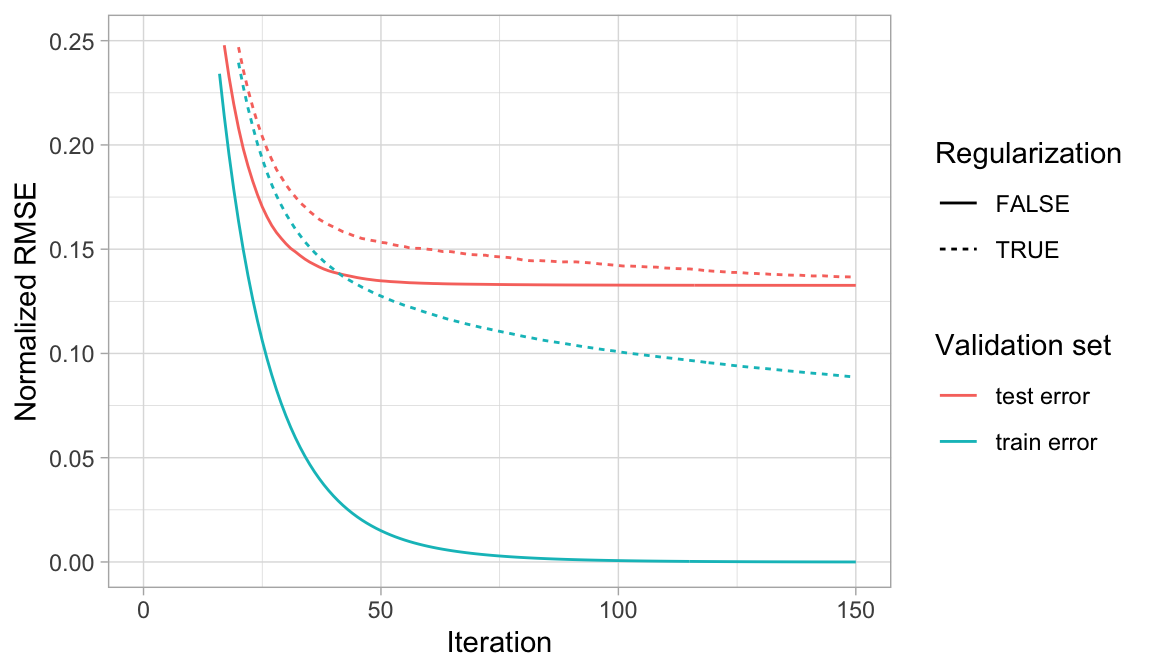
Figure 12.7: When a GBM model significantly overfits to the training data (blue), adding regularization (dotted line) causes the model to be more conservative on the training data, which can improve the cross-validated test error (red).
12.5.1.2 Dropout
Dropout is an alternative approach to reduce overfitting and can loosely be described as regularization. The dropout approach developed by Srivastava et al. (2014a) has been widely employed in deep learnings to prevent deep neural networks from overfitting (see Section 13.7.3). Dropout can also be used to address overfitting in GBMs. When constructing a GBM, the first few trees added at the beginning of the ensemble typically dominate the model performance while trees added later typically improve the prediction for only a small subset of the feature space. This often increases the risk of overfitting and the idea of dropout is to build an ensemble by randomly dropping trees in the boosting sequence. This is commonly referred to as DART (Rashmi and Gilad-Bachrach 2015) since it was initially explored in the context of Mutliple Additive Regression Trees (MART); DART refers to Dropout Additive Regression Trees. The percentage of dropouts is another regularization parameter.
Typically, when gamma, alpha, or lambda cannot help to control overfitting, exploring DART hyperparameters would be the next best option.33
12.5.2 Tuning strategy
The general tuning strategy for exploring xgboost hyperparameters builds onto the basic and stochastic GBM tuning strategies:
- Crank up the number of trees and tune learning rate with early stopping
- Tune tree-specific hyperparameters
- Explore stochastic GBM attributes
- If substantial overfitting occurs (e.g., large differences between train and CV error) explore regularization hyperparameters
- If you find hyperparameter values that are substantially different from default settings, be sure to retune the learning rate
- Obtain final “optimal” model
Running an XGBoost model with xgboost requires some additional data preparation. xgboost requires a matrix input for the features and the response to be a vector. Consequently, to provide a matrix input of the features we need to encode our categorical variables numerically (i.e. one-hot encoding, label encoding). The following numerically label encodes all categorical features and converts the training data frame to a matrix.
library(recipes)
xgb_prep <- recipe(Sale_Price ~ ., data = ames_train) %>%
  step_integer(all_nominal()) %>%
  prep(training = ames_train, retain = TRUE) %>%
  juice()

X <- as.matrix(xgb_prep[setdiff(names(xgb_prep), "Sale_Price")])
Y <- xgb_prep$Sale_Pricexgb.DMatrix objects. See ?xgboost::xgboost for details.
Next, we went through a series of grid searches similar to the previous sections and found the below model hyperparameters (provided via the params argument) to perform quite well. Our RMSE is slightly lower than the best regular and stochastic GBM models thus far.
set.seed(123)
ames_xgb <- xgb.cv(
  data = X,
  label = Y,
  nrounds = 6000,
  objective = "reg:linear",
  early_stopping_rounds = 50,
  nfold = 10,
  params = list(
    eta = 0.1,
    max_depth = 3,
    min_child_weight = 3,
    subsample = 0.8,
    colsample_bytree = 1.0),
  verbose = 0
)

# minimum test CV RMSE
min(ames_xgb$evaluation_log$test_rmse_mean)
## [1] 20488
Next, we assess if overfitting is limiting our model’s performance by performing a grid search that examines various regularization parameters (gamma, lambda, and alpha). Our results indicate that the best performing models use lambda equal to 1 and it doesn’t appear that alpha or gamma have any consistent patterns. However, even when lambda equals 1, our CV RMSE has no improvement over our previous XGBoost model.
Due to the low learning rate (eta), this cartesian grid search takes a long time. We stopped the search after 2 hours and only 98 of the 245 models had completed.
# hyperparameter grid
hyper_grid <- expand.grid(
  eta = 0.01,
  max_depth = 3,
  min_child_weight = 3,
  subsample = 0.5,
  colsample_bytree = 0.5,
  gamma = c(0, 1, 10, 100, 1000),
  lambda = c(0, 1e-2, 0.1, 1, 100, 1000, 10000),
  alpha = c(0, 1e-2, 0.1, 1, 100, 1000, 10000),
  rmse = 0,          # a place to dump RMSE results
  trees = 0          # a place to dump required number of trees
)

# grid search
for(i in seq_len(nrow(hyper_grid))) {
  set.seed(123)
  m <- xgb.cv(
    data = X,
    label = Y,
    nrounds = 4000,
    objective = "reg:linear",
    early_stopping_rounds = 50,
    nfold = 10,
    verbose = 0,
    params = list(
      eta = hyper_grid$eta[i],
      max_depth = hyper_grid$max_depth[i],
      min_child_weight = hyper_grid$min_child_weight[i],
      subsample = hyper_grid$subsample[i],
      colsample_bytree = hyper_grid$colsample_bytree[i],
      gamma = hyper_grid$gamma[i],
      lambda = hyper_grid$lambda[i],
      alpha = hyper_grid$alpha[i]
    )
  )
  hyper_grid$rmse[i] <- min(m$evaluation_log$test_rmse_mean)
  hyper_grid$trees[i] <- m$best_iteration
}

# results
hyper_grid %>%
  filter(rmse > 0) %>%
  arrange(rmse) %>%
  glimpse()
## Observations: 98
## Variables: 10
## $ eta              <dbl> 0.01, 0.01, 0.01, 0.01, 0.01, 0.0…
## $ max_depth        <dbl> 3, 3, 3, 3, 3, 3, 3, 3, 3, 3, 3, …
## $ min_child_weight <dbl> 3, 3, 3, 3, 3, 3, 3, 3, 3, 3, 3, …
## $ subsample        <dbl> 0.5, 0.5, 0.5, 0.5, 0.5, 0.5, 0.5…
## $ colsample_bytree <dbl> 0.5, 0.5, 0.5, 0.5, 0.5, 0.5, 0.5…
## $ gamma            <dbl> 0, 1, 10, 100, 1000, 0, 1, 10, 10…
## $ lambda           <dbl> 1, 1, 1, 1, 1, 1, 1, 1, 1, 1, 1, …
## $ alpha            <dbl> 0.00, 0.00, 0.00, 0.00, 0.00, 0.1…
## $ rmse             <dbl> 20488, 20488, 20488, 20488, 20488…
## $ trees            <dbl> 3944, 3944, 3944, 3944, 3944, 381…
Once you’ve found the optimal hyperparameters, fit the final model with xgb.train or xgboost. Be sure to use the optimal number of trees found during cross validation. In our example, adding regularization provides no improvement so we exclude them in our final model.
# optimal parameter list
params <- list(
  eta = 0.01,
  max_depth = 3,
  min_child_weight = 3,
  subsample = 0.5,
  colsample_bytree = 0.5
)

# train final model
xgb.fit.final <- xgboost(
  params = params,
  data = X,
  label = Y,
  nrounds = 3944,
  objective = "reg:linear",
  verbose = 0
)
12.6 Feature interpretation
Measuring GBM feature importance and effects follows the same construct as random forests. Similar to random forests, the gbm and h2o packages offer an impurity-based feature importance. xgboost actually provides three built-in measures for feature importance:
- Gain: This is equivalent to the impurity measure in random forests (reference Section 11.6) and is the most common model-centric metric to use.
- Coverage: The Coverage metric quantifies the relative number of observations influenced by this feature. For example, if you have 100 observations, 4 features and 3 trees, and suppose \(x_1\) is used to decide the leaf node for 10, 5, and 2 observations in \(tree_1\), \(tree_2\) and \(tree_3\) respectively; then the metric will count cover for this feature as \(10+5+2 = 17\) observations. This will be calculated for all the 4 features and expressed as a percentage.
- Frequency: The percentage representing the relative number of times a particular feature occurs in the trees of the model. In the above example, if \(x_1\) was used for 2 splits, 1 split and 3 splits in each of \(tree_1\), \(tree_2\) and \(tree_3\) respectively; then the weightage for \(x_1\) will be \(2+1+3=6\). The frequency for \(x_1\) is calculated as its percentage weight over weights of all \(x_p\) features.
If we examine the top 10 influential features in our final model using the impurity (gain) metric, we see very similar results as we saw with our random forest model (Section 11.6). The primary difference is we no longer see Neighborhood as a top influential feature, which is likely a result of how we label encoded the categorical features.
By default, vip::vip() uses the gain method for feature importance but you can assess the other types using the type argument. You can also use xgboost::xgb.ggplot.importance() to plot the various feature importance measures but you need to first run xgb.importance() on the final model.
# variable importance plot
vip::vip(xgb.fit.final) 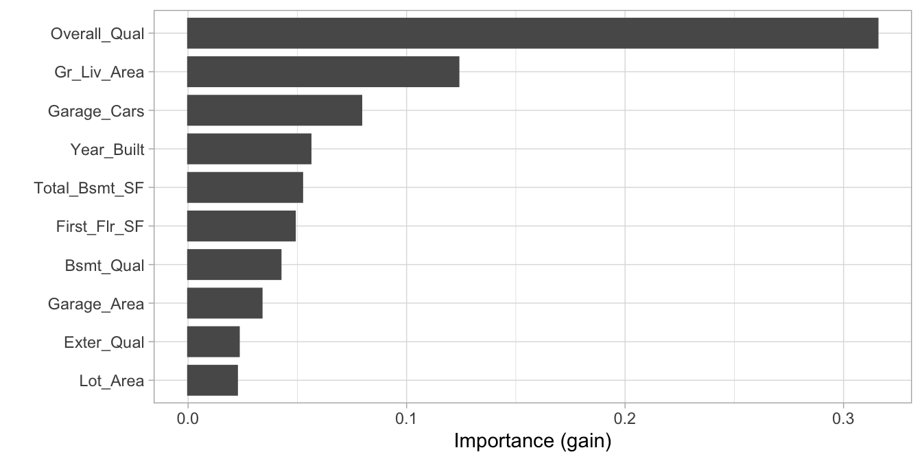
Figure 12.8: Top 10 most important variables based on the impurity (gain) metric.
12.7 Final thoughts
GBMs are one of the most powerful ensemble algorithms that are often first-in-class with predictive accuracy. Although they are less intuitive and more computationally demanding than many other machine learning algorithms, they are essential to have in your toolbox.
Although we discussed the most popular GBM algorithms, realize there are alternative algorithms not covered here. For example LightGBM (Ke et al. 2017) is a gradient boosting framework that focuses on leaf-wise tree growth versus the traditional level-wise tree growth. This means as a tree is grown deeper, it focuses on extending a single branch versus growing multiple branches (reference Figure 9.2. CatBoost (Dorogush, Ershov, and Gulin 2018) is another gradient boosting framework that focuses on using efficient methods for encoding categorical features during the gradient boosting process. Both frameworks are available in R.
References
Breiman, Leo. 1996a. “Bagging Predictors.” Machine Learning 24 (2). Springer: 123–40.
Breiman, Leo. 2001. “Random Forests.” Machine Learning 45 (1). Springer: 5–32.
Chen, Tianqi, and Carlos Guestrin. 2016. “XGBoost: A Scalable Tree Boosting System.” In Proceedings of the 22nd Acm Sigkdd International Conference on Knowledge Discovery and Data Mining, 785–94. KDD ’16. New York, NY, USA: ACM. https://doi.org/10.1145/2939672.2939785.
Chen, Tianqi, Tong He, Michael Benesty, Vadim Khotilovich, Yuan Tang, Hyunsu Cho, Kailong Chen, et al. 2018. Xgboost: Extreme Gradient Boosting. https://CRAN.R-project.org/package=xgboost.
Dorogush, Anna Veronika, Vasily Ershov, and Andrey Gulin. 2018. “CatBoost: Gradient Boosting with Categorical Features Support.” arXiv Preprint arXiv:1810.11363.
Freund, Yoav, and Robert E Schapire. 1999. “Adaptive Game Playing Using Multiplicative Weights.” Games and Economic Behavior 29 (1-2). Elsevier: 79–103.
Friedman, Jerome H. 2001. “Greedy Function Approximation: A Gradient Boosting Machine.” Annals of Statistics. JSTOR, 1189–1232.
Friedman, Jerome H. 2002. “Stochastic Gradient Boosting.” Computational Statistics & Data Analysis 38 (4). Elsevier: 367–78.
Friedman, Jerome, Trevor Hastie, and Robert Tibshirani. 2001. The Elements of Statistical Learning. Vol. 1. Springer Series in Statistics New York, NY, USA:
Greenwell, B, B Boehmke, J Cunningham, and GBM Developers. 2018. “Gbm: Generalized Boosted Regression Models.” R Package Version 2.1 4.
Ke, Guolin, Qi Meng, Thomas Finley, Taifeng Wang, Wei Chen, Weidong Ma, Qiwei Ye, and Tie-Yan Liu. 2017. “Lightgbm: A Highly Efficient Gradient Boosting Decision Tree.” In Advances in Neural Information Processing Systems, 3146–54.
Kuhn, Max, and Kjell Johnson. 2013. Applied Predictive Modeling. Vol. 26. Springer.
Probst, Philipp, Bernd Bischl, and Anne-Laure Boulesteix. 2018. “Tunability: Importance of Hyperparameters of Machine Learning Algorithms.” arXiv Preprint arXiv:1802.09596.
Rashmi, Korlakai Vinayak, and Ran Gilad-Bachrach. 2015. “DART: Dropouts Meet Multiple Additive Regression Trees.” In AISTATS, 489–97.
Srivastava, Nitish, Geoffrey Hinton, Alex Krizhevsky, Ilya Sutskever, and Ruslan Salakhutdinov. 2014a. “Dropout: A Simple Way to Prevent Neural Networks from Overfitting.” Journal of Machine Learning Research 15: 1929–58. http://jmlr.org/papers/v15/srivastava14a.html.