Chapter 10 Bagging

In Section 2.4.2 we learned about bootstrapping as a resampling procedure, which creates b new bootstrap samples by drawing samples with replacement of the original training data. This chapter illustrates how we can use bootstrapping to create an ensemble of predictions. Bootstrap aggregating, also called bagging, is one of the first ensemble algorithms²⁸ machine learning practitioners learn and is designed to improve the stability and accuracy of regression and classification algorithms. By model averaging, bagging helps to reduce variance and minimize overfitting. Although it is usually applied to decision tree methods, it can be used with any type of method.

10.1 Prerequisites

In this chapter we’ll make use of the following packages:

# Helper packages
library(dplyr)       # for data wrangling
library(ggplot2)     # for awesome plotting
library(doParallel)  # for parallel backend to foreach
library(foreach)     # for parallel processing with for loops

# Modeling packages
library(caret)       # for general model fitting
library(rpart)       # for fitting decision trees
library(ipred)       # for fitting bagged decision trees

We’ll continue to illustrate the main concepts with the ames_train data set created in Section 2.7.

10.2 Why and when bagging works

Bootstrap aggregating (bagging) prediction models is a general method for fitting multiple versions of a prediction model and then combining (or ensembling) them into an aggregated prediction (Breiman 1996a). Bagging is a fairly straight forward algorithm in which b bootstrap copies of the original training data are created, the regression or classification algorithm (commonly referred to as the base learner) is applied to each bootstrap sample and, in the regression context, new predictions are made by averaging the predictions together from the individual base learners. When dealing with a classification problem, the base learner predictions are combined using plurality vote or by averaging the estimated class probabilities together. This is represented in Equation (10.1) where \(X\) is the record for which we want to generate a prediction, \(\widehat{f_{bag}}\) is the bagged prediction, and \(\widehat{f_1}\left(X\right), \widehat{f_2}\left(X\right), \dots, \widehat{f_b}\left(X\right)\) are the predictions from the individual base learners.

\[\begin{equation} \tag{10.1} \widehat{f_{bag}} = \widehat{f_1}\left(X\right) + \widehat{f_2}\left(X\right) + \cdots + \widehat{f_b}\left(X\right) \end{equation}\]

Because of the aggregation process, bagging effectively reduces the variance of an individual base learner (i.e., averaging reduces variance); however, bagging does not always improve upon an individual base learner. As discussed in Section 2.5, some models have larger variance than others. Bagging works especially well for unstable, high variance base learners—algorithms whose predicted output undergoes major changes in response to small changes in the training data (Dietterich 2000b, 2000a). This includes algorithms such as decision trees and KNN (when k is sufficiently small). However, for algorithms that are more stable or have high bias, bagging offers less improvement on predicted outputs since there is less variability (e.g., bagging a linear regression model will effectively just return the original predictions for large enough \(b\)).

The general idea behind bagging is referred to as the “wisdom of the crowd” effect and was popularized by Surowiecki (2005). It essentially means that the aggregation of information in large diverse groups results in decisions that are often better than could have been made by any single member of the group. The more diverse the group members are then the more diverse their perspectives and predictions will be, which often leads to better aggregated information. Think of estimating the number of jelly beans in a jar at a carinival. While any individual guess is likely to be way off, you’ll often find that the averaged guesses tends to be a lot closer to the true number.

This is illustrated in Figure 10.1, which compares bagging \(b = 100\) polynomial regression models, MARS models, and CART decision trees. You can see that the low variance base learner (polynomial regression) gains very little from bagging while the higher variance learner (decision trees) gains significantly more. Not only does bagging help minimize the high variability (instability) of single trees, but it also helps to smooth out the prediction surface.

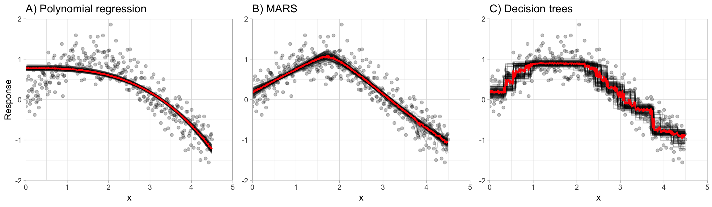
Figure 10.1: The effect of bagging 100 base learners. High variance models such as decision trees (C) benefit the most from the aggregation effect in bagging, whereas low variance models such as polynomial regression (A) show little improvement.

Optimal performance is often found by bagging 50–500 trees. Data sets that have a few strong predictors typically require less trees; whereas data sets with lots of noise or multiple strong predictors may need more. Using too many trees will not lead to overfitting. However, it’s important to realize that since multiple models are being run, the more iterations you perform the more computational and time requirements you will have. As these demands increase, performing k-fold CV can become computationally burdensome.

A benefit to creating ensembles via bagging, which is based on resampling with replacement, is that it can provide its own internal estimate of predictive performance with the out-of-bag (OOB) sample (see Section 2.4.2). The OOB sample can be used to test predictive performance and the results usually compare well compared to k-fold CV assuming your data set is sufficiently large (say \(n \geq 1,000\)). Consequently, as your data sets become larger and your bagging iterations increase, it is common to use the OOB error estimate as a proxy for predictive performance.

Think of the OOB estimate of generalization performance as an unstructured, but free CV statistic.

10.3 Implementation

In Chapter 9, we saw how decision trees performed in predicting the sales price for the Ames housing data. Performance was subpar compared to the MARS (Chapter 7) and KNN (Chapter 8) models we fit, even after tuning to find the optimal pruned tree. Rather than use a single pruned decision tree, we can use, say, 100 bagged unpruned trees (by not pruning the trees we’re keeping bias low and variance high which is when bagging will have the biggest effect). As the below code chunk illustrates, we gain significant improvement over our individual (pruned) decision tree (RMSE of 26,462 for bagged trees vs. 41,019 for the single decision tree).

The bagging() function comes from the ipred package and we use nbagg to control how many iterations to include in the bagged model and coob = TRUE indicates to use the OOB error rate. By default, bagging() uses rpart::rpart() for decision tree base learners but other base learners are available. Since bagging just aggregates a base learner, we can tune the base learner parameters as normal. Here, we pass parameters to rpart() with the control parameter and we build deep trees (no pruning) that require just two observations in a node to split.

# make bootstrapping reproducible
set.seed(123)

# train bagged model
ames_bag1 <- bagging(
  formula = Sale_Price ~ .,
  data = ames_train,
  nbagg = 100,  
  coob = TRUE,
  control = rpart.control(minsplit = 2, cp = 0)
)

ames_bag1
## 
## Bagging regression trees with 100 bootstrap replications 
## 
## Call: bagging.data.frame(formula = Sale_Price ~ ., data = ames_train, 
##     nbagg = 100, coob = TRUE, control = rpart.control(minsplit = 2, 
##         cp = 0))
## 
## Out-of-bag estimate of root mean squared error:  25528.78

One thing to note is that typically, the more trees the better. As we add more trees we’re averaging over more high variance decision trees. Early on, we see a dramatic reduction in variance (and hence our error) but eventually the error will typically flatline and stabilize signaling that a suitable number of trees has been reached. Often, we need only 50–100 trees to stabilize the error (in other cases we may need 500 or more). For the Ames data we see that the error is stabilizing with just over 100 trees so we’ll likely not gain much improvement by simply bagging more trees.

Unfortunately, bagging() does not provide the RMSE by tree so to produce this error curve we iterated over nbagg values of 1–200 and applied the same bagging() function above.

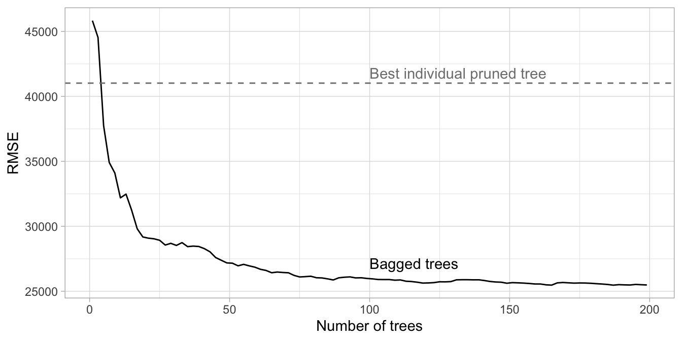
Figure 10.2: Error curve for bagging 1-200 deep, unpruned decision trees. The benefit of bagging is optimized at 187 trees although the majority of error reduction occurred within the first 100 trees.

We can also apply bagging within caret and use 10-fold CV to see how well our ensemble will generalize. We see that the cross-validated RMSE for 200 trees is similar to the OOB estimate (difference of 495). However, using the OOB error took 58 seconds to compute whereas performing the following 10-fold CV took roughly 26 minutes on our machine!

ames_bag2 <- train(
  Sale_Price ~ .,
  data = ames_train,
  method = "treebag",
  trControl = trainControl(method = "cv", number = 10),
  nbagg = 200,  
  control = rpart.control(minsplit = 2, cp = 0)
)
ames_bag2
## Bagged CART 
## 
## 2054 samples
##   80 predictor
## 
## No pre-processing
## Resampling: Cross-Validated (10 fold) 
## Summary of sample sizes: 1849, 1848, 1848, 1849, 1849, 1847, ... 
## Resampling results:
## 
##   RMSE      Rsquared   MAE     
##   26957.06  0.8900689  16713.14

10.4 Easily parallelize

As stated in Section 10.2, bagging can become computationally intense as the number of iterations increases. Fortunately, the process of bagging involves fitting models to each of the bootstrap samples which are completely independent of one another. This means that each model can be trained in parallel and the results aggregated in the end for the final model. Consequently, if you have access to a large cluster or number of cores, you can more quickly create bagged ensembles on larger data sets.

The following illustrates parallelizing the bagging algorithm (with \(b = 160\) decision trees) on the Ames housing data using eight cores and returning the predictions for the test data for each of the trees.

# Create a parallel socket cluster
cl <- makeCluster(8) # use 8 workers
registerDoParallel(cl) # register the parallel backend

# Fit trees in parallel and compute predictions on the test set
predictions <- foreach(
  icount(160), 
  .packages = "rpart", 
  .combine = cbind
  ) %dopar% {
    # bootstrap copy of training data
    index <- sample(nrow(ames_train), replace = TRUE)
    ames_train_boot <- ames_train[index, ]  
  
    # fit tree to bootstrap copy
    bagged_tree <- rpart(
      Sale_Price ~ ., 
      control = rpart.control(minsplit = 2, cp = 0),
      data = ames_train_boot
      ) 
    
    predict(bagged_tree, newdata = ames_test)
}

predictions[1:5, 1:7]
##   result.1 result.2 result.3 result.4 result.5 result.6 result.7
## 1   176500   187000   179900   187500   187500   187500   187500
## 2   180000   254000   251000   240000   180000   180000   221000
## 3   175000   174000   192000   192000   185000   178900   163990
## 4   197900   157000   217500   215000   180000   210000   218500
## 5   120000   129000   130000   143000   136500   153600   148500

We can then do some data wrangling to compute and plot the RMSE as additional trees are added. Our results, illustrated in Figure 10.3, closely resemble the results obtained in Figure 10.2. This also illustrates how the OOB error closely approximates the test error.

predictions %>%
  as.data.frame() %>%
  mutate(
    observation = 1:n(),
    actual = ames_test$Sale_Price) %>%
  tidyr::gather(tree, predicted, -c(observation, actual)) %>%
  group_by(observation) %>%
  mutate(tree = stringr::str_extract(tree, '\\d+') %>% as.numeric()) %>%
  ungroup() %>%
  arrange(observation, tree) %>%
  group_by(observation) %>%
  mutate(avg_prediction = cummean(predicted)) %>%
  group_by(tree) %>%
  summarize(RMSE = RMSE(avg_prediction, actual)) %>%
  ggplot(aes(tree, RMSE)) +
  geom_line() +
  xlab('Number of trees')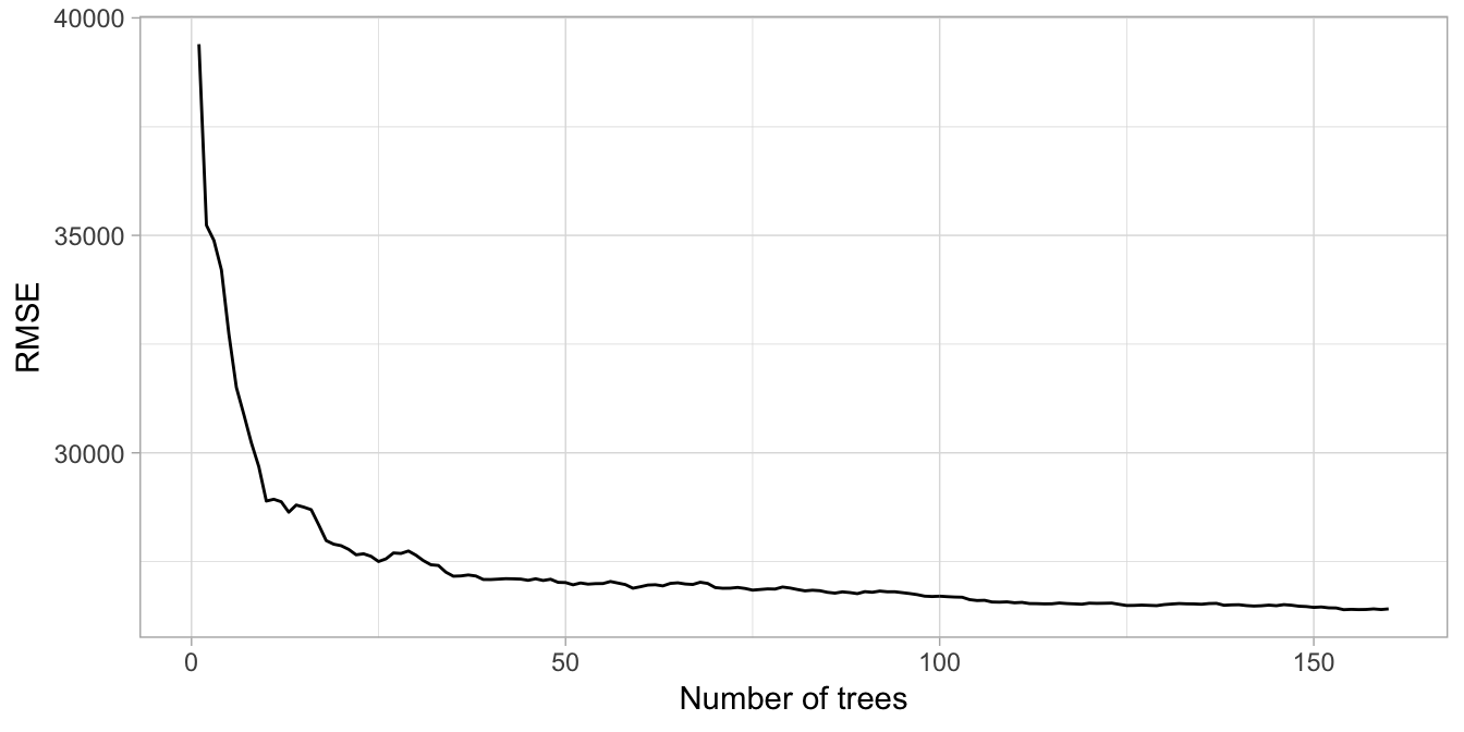

Figure 10.3: Error curve for custom parallel bagging of 1-160 deep, unpruned decision trees.

# Shutdown parallel cluster
stopCluster(cl)

10.5 Feature interpretation

Unfortunately, due to the bagging process, models that are normally perceived as interpretable are no longer so. However, we can still make inferences about how features are influencing our model. Recall in Section 9.6 that we measure feature importance based on the sum of the reduction in the loss function (e.g., SSE) attributed to each variable at each split in a given tree.

For bagged decision trees, this process is similar. For each tree, we compute the sum of the reduction of the loss function across all splits. We then aggregate this measure across all trees for each feature. The features with the largest average decrease in SSE (for regression) are considered most important. Unfortunately, the ipred package does not capture the required information for computing variable importance but the caret package does. In the code chunk below, we use vip to construct a variable importance plot (VIP) of the top 40 features in the ames_bag2 model.

With a single decision tree, we saw that many non-informative features were not used in the tree. However, with bagging, since we use many trees built on bootstrapped samples, we are likely to see many more features used for splits. Consequently, we tend to have many more features involved but with lower levels of importance.

vip::vip(ames_bag2, num_features = 40, bar = FALSE)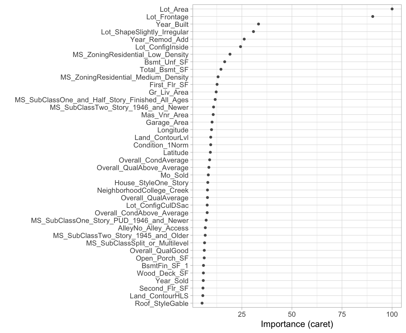

Figure 10.4: Variable importance for 200 bagged trees for the Ames Housing data.

Understanding the relationship between a feature and predicted response for bagged models follows the same procedure we’ve seen in previous chapters. PDPs tell us visually how each feature influences the predicted output, on average. Although the averaging effect of bagging diminishes the ability to interpret the final ensemble, PDPs and other interpretability methods (Chapter 16) help us to interpret any “black box” model. Figure 10.5 highlights the unique, and sometimes non-linear, non-monotonic relationships that may exist between a feature and response.

# Construct partial dependence plots
p1 <- pdp::partial(
  ames_bag2, 
  pred.var = "Lot_Area",
  grid.resolution = 20
  ) %>% 
  autoplot()

p2 <- pdp::partial(
  ames_bag2, 
  pred.var = "Lot_Frontage", 
  grid.resolution = 20
  ) %>% 
  autoplot()

gridExtra::grid.arrange(p1, p2, nrow = 1)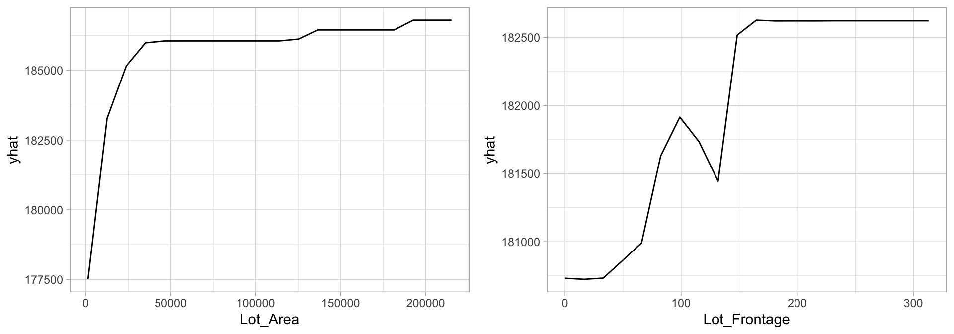

Figure 10.5: Partial dependence plots to understand the relationship between sales price and the lot area and frontage size features.

10.6 Final thoughts

Bagging improves the prediction accuracy for high variance (and low bias) models at the expense of interpretability and computational speed. However, using various interpretability algorithms such as VIPs and PDPs, we can still make inferences about how our bagged model leverages feature information. Also, since bagging consists of independent processes, the algorithm is easily parallelizable.

However, when bagging trees, a problem still exists. Although the model building steps are independent, the trees in bagging are not completely independent of each other since all the original features are considered at every split of every tree. Rather, trees from different bootstrap samples typically have similar structure to each other (especially at the top of the tree) due to any underlying strong relationships.

For example, if we create six decision trees with different bootstrapped samples of the Boston housing data (Harrison Jr and Rubinfeld 1978), we see a similar structure as the top of the trees. Although there are 15 predictor variables to split on, all six trees have both lstat and rm variables driving the first few splits.

We use the Boston housing data in this example because it has fewer features and shorter names than the Ames housing data. Consequently, it is easier to compare multiple trees side-by-side; however, the same tree correlation problem exists in the Ames bagged model.

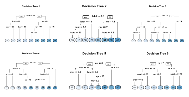
Figure 10.6: Six decision trees based on different bootstrap samples.

This characteristic is known as tree correlation and prevents bagging from further reducing the variance of the base learner. In the next chapter, we discuss how random forests extend and improve upon bagged decision trees by reducing this correlation and thereby improving the accuracy of the overall ensemble.

References

Breiman, Leo. 1996a. “Bagging Predictors.” Machine Learning 24 (2). Springer: 123–40.

Dietterich, Thomas G. 2000a. “An Experimental Comparison of Three Methods for Constructing Ensembles of Decision Trees: Bagging, Boosting, and Randomization.” Machine Learning 40 (2). Springer: 139–57.

Dietterich, Thomas G. 2000b. “Ensemble Methods in Machine Learning.” In International Workshop on Multiple Classifier Systems, 1–15. Springer.

Harrison Jr, David, and Daniel L Rubinfeld. 1978. “Hedonic Housing Prices and the Demand for Clean Air.” Journal of Environmental Economics and Management 5 (1). Elsevier: 81–102.

Surowiecki, James. 2005. The Wisdom of Crowds. Anchor.

---

28. Also commonly referred to as a meta-algorithm.↩