Chapter 13 Deep Learning

Machine learning algorithms typically search for the optimal representation of data using a feedback signal in the form of an objective function. However, most machine learning algorithms only have the ability to use one or two layers of data transformation to learn the output representation. We call these shallow models³⁴ since they only use 1–2 representations of the feature space. As data sets continue to grow in the dimensions of the feature space, finding the optimal output representation with a shallow model is not always possible. Deep learning provides a multi-layer approach to learn data representations, typically performed with a multi-layer neural network. Like other machine learning algorithms, deep neural networks (DNN) perform learning by mapping features to targets through a process of simple data transformations and feedback signals; however, DNNs place an emphasis on learning successive layers of meaningful representations. Although an intimidating subject, the overarching concept is rather simple and has proven highly successful across a wide range of problems (e.g., image classification, speech recognition, autonomous driving). This chapter will teach you the fundamentals of building a simple feedforward DNN, which is the foundation for the more advanced deep learning models.

Our online resources will provide content covering additional deep learning models such as convolutional, recurrent, and long short-term memory neural networks. Moreover, Chollet and Allaire (2018) is an excellent, in-depth text on applying deep learning methods with R.

13.1 Prerequisites

This tutorial will use a few supporting packages but the main emphasis will be on the keras package (Allaire and Chollet 2019). Additional content provided online illustrates how to execute the same procedures we cover here with the h2o package. For more information on installing both CPU and GPU-based Keras and TensorFlow software, visit https://keras.rstudio.com.

# Helper packages
library(dplyr)         # for basic data wrangling

# Modeling packages
library(keras)         # for fitting DNNs
library(tfruns)        # for additional grid search & model training functions

# Modeling helper package - not necessary for reproducibility
library(tfestimators)  # provides grid search & model training interface

We’ll use the MNIST data to illustrate various DNN concepts. With DNNs, it is important to note a few items:

Feedforward DNNs require all feature inputs to be numeric. Consequently, if your data contains categorical features they will need to be numerically encoded (e.g., one-hot encoded, integer label encoded, etc.).
Due to the data transformation process that DNNs perform, they are highly sensitive to the individual scale of the feature values. Consequently, we should standardize our features first. Although the MNIST features are measured on the same scale (0–255), they are not standardized (i.e., have mean zero and unit variance); the code chunk below standardizes the MNIST data to resolve this.³⁵
Since we are working with a multinomial response (0–9), keras requires our response to be a one-hot encoded matrix, which can be accomplished with the keras function to_categorical().

# Import MNIST training data
mnist <- dslabs::read_mnist()
mnist_x <- mnist$train$images
mnist_y <- mnist$train$labels

# Rename columns and standardize feature values
colnames(mnist_x) <- paste0("V", 1:ncol(mnist_x))
mnist_x <- mnist_x / 255

# One-hot encode response
mnist_y <- to_categorical(mnist_y, 10)

13.2 Why deep learning

Neural networks originated in the computer science field to answer questions that normal statistical approaches were not designed to answer at the time. The MNIST data is one of the most common examples you will find, where the goal is to to analyze hand-written digits and predict the numbers written. This problem was originally presented to AT&T Bell Lab’s to help build automatic mail-sorting machines for the USPS (LeCun et al. 1990).

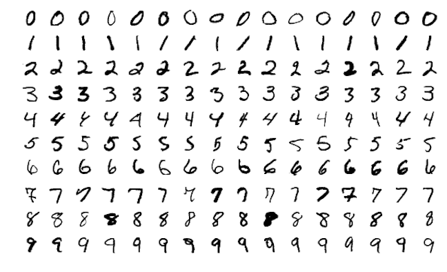
$Sample images from MNIST test dataset \citep{wikiMNIST}.$

Figure 13.1: Sample images from MNIST test dataset .

This problem is quite unique because many different features of the data can be represented. As humans, we look at these numbers and consider features such as angles, edges, thickness, completeness of circles, etc. We interpret these different representations of the features and combine them to recognize the digit. In essence, neural networks perform the same task albeit in a far simpler manner than our brains. At their most basic levels, neural networks have three layers: an input layer, a hidden layer, and an output layer. The input layer consists of all of the original input features. The majority of the learning takes place in the hidden layer, and the output layer outputs the final predictions.

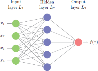
Figure 13.2: Representation of a simple feedforward neural network.

Although simple on the surface, the computations being performed inside a network require lots of data to learn and are computationally intense rendering them impractical to use in the earlier days. However, over the past several decades, advancements in computer hardware (off the shelf CPUs became faster and GPUs were created) made the computations more practical, the growth in data collection made them more relevant, and advancements in the underlying algorithms made the depth (number of hidden layers) of neural nets less of a constraint. These advancements have resulted in the ability to run very deep and highly parameterized neural networks (i.e., DNNs).

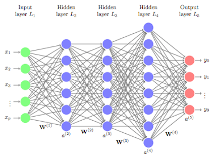
Figure 13.3: Representation of a deep feedforward neural network.

Such DNNs allow for very complex representations of data to be modeled, which has opened the door to analyzing high-dimensional data (e.g., images, videos, and sound bytes). In some machine learning approaches, features of the data need to be defined prior to modeling (e.g., ordinary linear regression). One can only imagine trying to create the features for the digit recognition problem above. However, with DNNs, the hidden layers provide the means to auto-identify useful features. A simple way to think of this is to go back to our digit recognition problem. The first hidden layer may learn about the angles of the line, the next hidden layer may learn about the thickness of the lines, the next may learn the location and completeness of the circles, etc. Aggregating these different attributes together by linking the layers allows the model to accurately predict what digit each image represents.

This is the reason that DNNs are so popular for very complex problems where feature engineering is important, but rather difficult to do by hand (e.g., facial recognition). However, at their core, DNNs perform successive non-linear transformations across each layer, allowing DNNs to model very complex and non-linear relationships. This can make DNNs suitable machine learning approaches for traditional regression and classification problems as well. But it is important to keep in mind that deep learning thrives when dimensions of your data are sufficiently large (e.g., very large training sets). As the number of observations ($n$) and feature inputs ($p$) decrease, shallow machine learning approaches tend to perform just as well, if not better, and are more efficient.

13.3 Feedforward DNNs

Multiple DNN architectures exist and, as interest and research in this area increases, the field will continue to flourish. For example, convolutional neural networks (CNNs or ConvNets) have widespread applications in image and video recognition, recurrent neural networks (RNNs) are often used with speech recognition, and long short-term memory neural networks (LSTMs) are advancing automated robotics and machine translation. However, fundamental to all these methods is the feedforward DNN (aka multilayer perceptron). Feedforward DNNs are densely connected layers where inputs influence each successive layer which then influences the final output layer.

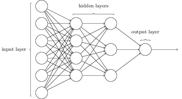
Figure 13.4: Feedforward neural network.

To build a feedforward DNN we need four key components:

Input data ✔
A pre-defined network architecture;
A feedback mechanism to help the network learn;
A model training approach.

The next few sections will walk you through steps 2)–4) to build a feedforward DNN to the MNIST data.

13.4 Network architecture

When developing the network architecture for a feedforward DNN, you really only need to worry about two features: (1) layers and nodes, and (2) activation.

13.4.1 Layers and nodes

The layers and nodes are the building blocks of our DNN and they decide how complex the network will be. Layers are considered dense (fully connected) when all the nodes in each successive layer are connected. Consequently, the more layers and nodes you add the more opportunities for new features to be learned (commonly referred to as the model’s capacity).³⁶ Beyond the input layer, which is just our original predictor variables, there are two main types of layers to consider: hidden layers and an output layer.

13.4.1.1 Hidden layers

There is no well-defined approach for selecting the number of hidden layers and nodes; rather, these are the first of many hyperparameters to tune. With regular tabular data, 2–5 hidden layers are often sufficient but your best bet is to err on the side of more layers rather than fewer. The number of nodes you incorporate in these hidden layers is largely determined by the number of features in your data. Often, the number of nodes in each layer is equal to or less than the number of features but this is not a hard requirement. It is important to note that the number of hidden layers and nodes in your network can affect its computational complexity (e.g., training time). When dealing with many features and, therefore, many nodes, training deep models with many hidden layers can be computationally more efficient than training a single layer network with the same number of high volume nodes (Goodfellow, Bengio, and Courville 2016). Consequently, the goal is to find the simplest model with optimal performance.

13.4.1.2 Output layers

The choice of output layer is driven by the modeling task. For regression problems, your output layer will contain one node that outputs the final predicted value. Classification problems are different. If you are predicting a binary output (e.g., True/False, Win/Loss), your output layer will still contain only one node and that node will predict the probability of success (however you define success). However, if you are predicting a multinomial output, the output layer will contain the same number of nodes as the number of classes being predicted. For example, in our MNIST data, we are predicting 10 classes (0–9); therefore, the output layer will have 10 nodes and the output would provide the probability of each class.

13.4.1.3 Implementation

The keras package allows us to develop our network with a layering approach. First, we initiate our sequential feedforward DNN architecture with keras_model_sequential() and then add some dense layers. This example creates two hidden layers, the first with 128 nodes and the second with 64, followed by an output layer with 10 nodes. One thing to point out is that the first layer needs the input_shape argument to equal the number of features in your data; however, the successive layers are able to dynamically interpret the number of expected inputs based on the previous layer.

model <- keras_model_sequential() %>%
  layer_dense(units = 128, input_shape = ncol(mnist_x)) %>%
  layer_dense(units = 64) %>%
  layer_dense(units = 10)

13.4.2 Activation

A key component with neural networks is what’s called activation. In the human brain, the biologic neuron receives inputs from many adjacent neurons. When these inputs accumulate beyond a certain threshold the neuron is activated suggesting there is a signal. DNNs work in a similar fashion.

13.4.2.1 Activation functions

As stated previously, each node is connected to all the nodes in the previous layer. Each connection gets a weight and then that node adds all the incoming inputs multiplied by its corresponding connection weight plus an extra bias parameter ($w_0$). The summed total of these inputs become an input to an activation function; see 13.5.

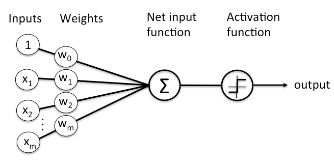
Figure 13.5: Flow of information in an artificial neuron.

The activation function is simply a mathematical function that determines whether or not there is enough informative input at a node to fire a signal to the next layer. There are multiple activation functions to choose from but the most common ones include:

\[\begin{equation} \tag{13.1} \texttt{Linear (identity):} \;\; f\left(x\right) = x \end{equation}\]

\[\begin{equation} \tag{13.2} \texttt{Rectified linear unit (ReLU):} \;\; f\left(x\right) = \begin{cases} 0, & \text{for $x<0$}.\\ x, & \text{for $x\geq0$}. \end{cases} \end{equation}\]

\[\begin{equation} \tag{13.3} \texttt{Sigmoid:} \;\; f\left(x\right) = \frac{1}{1 + e^{-x}} \end{equation}\]

\[\begin{equation} \tag{13.4} \texttt{Softmax:} \;\; f\left(x\right) = \frac{e^{x_i}}{\sum_j e^{x_j}} \end{equation}\]

When using rectangular data, the most common approach is to use ReLU activation functions in the hidden layers. The ReLU activation function is simply taking the summed weighted inputs and transforming them to a $0$ (not fire) or $>0$ (fire) if there is enough signal. For the output layers we use the linear activation function for regression problems, the sigmoid activation function for binary classification problems, and softmax for multinomial classification problems.

13.4.2.2 Implementation

To control the activation functions used in our layers we specify the activation argument. For the two hidden layers we add the ReLU activation function and for the output layer we specify activation = softmax (since MNIST is a multinomial classification problem).

model <- keras_model_sequential() %>%
  layer_dense(units = 128, activation = "relu", input_shape = p) %>%
  layer_dense(units = 64, activation = "relu") %>%
  layer_dense(units = 10, activation = "softmax")

Next, we need to incorporate a feedback mechanism to help our model learn.

13.5 Backpropagation

On the first run (or forward pass), the DNN will select a batch of observations, randomly assign weights across all the node connections, and predict the output. The engine of neural networks is how it assesses its own accuracy and automatically adjusts the weights across all the node connections to improve that accuracy. This process is called backpropagation. To perform backpropagation we need two things:

An objective function;
An optimizer.

First, you need to establish an objective (loss) function to measure performance. For regression problems this might be mean squared error (MSE) and for classification problems it is commonly binary and multi-categorical cross entropy (reference Section 2.6). DNNs can have multiple loss functions but we’ll just focus on using one.

On each forward pass the DNN will measure its performance based on the loss function chosen. The DNN will then work backwards through the layers, compute the gradient³⁷ of the loss with regards to the network weights, adjust the weights a little in the opposite direction of the gradient, grab another batch of observations to run through the model, …rinse and repeat until the loss function is minimized. This process is known as mini-batch stochastic gradient descent³⁸ (mini-batch SGD). There are several variants of mini-batch SGD algorithms; they primarily differ in how fast they descend the gradient (controlled by the learning rate as discussed in Section 12.2.2). These different variations make up the different optimizers that can be used.

Understanding the technical differences among the variants of gradient descent is beyond the intent of this book. An excellent source to learn more about these differences and appropriate scenarios to adjust this parameter is provided by Ruder (2016). For now, realize that sticking with the default optimizer (RMSProp) is often sufficient for most normal regression and classification problems; however, this is a tunable hyperparameter.

To incorporate the backpropagation piece of our DNN we include compile() in our code sequence. In addition to the optimizer and loss function arguments, we can also identify one or more metrics in addition to our loss function to track and report.

model <- keras_model_sequential() %>%
  
  # Network architecture
  layer_dense(units = 128, activation = "relu", input_shape = ncol(mnist_x)) %>%
  layer_dense(units = 64, activation = "relu") %>%
  layer_dense(units = 10, activation = "softmax") %>%
  
  # Backpropagation
  compile(
    loss = 'categorical_crossentropy',
    optimizer = optimizer_rmsprop(),
    metrics = c('accuracy')
  )

13.6 Model training

We’ve created a base model, now we just need to train it with some data. To do so we feed our model into a fit() function along with our training data. We also provide a few other arguments that are worth mentioning:

batch_size: As we mentioned in the last section, the DNN will take a batch of data to run through the mini-batch SGD process. Batch sizes can be between one and several hundred. Small values will be more computationally burdensome while large values provide less feedback signal. Values are typically provided as a power of two that fit nicely into the memory requirements of the GPU or CPU hardware like 32, 64, 128, 256, and so on.
epochs: An epoch describes the number of times the algorithm sees the entire data set. So, each time the algorithm has seen all samples in the data set, an epoch has completed. In our training set, we have 60,000 observations so running batches of 128 will require 469 passes for one epoch. The more complex the features and relationships in your data, the more epochs you’ll require for your model to learn, adjust the weights, and minimize the loss function.
validation_split: The model will hold out XX% of the data so that we can compute a more accurate estimate of an out-of-sample error rate.
verbose: We set this to FALSE for brevity; however, when TRUE you will see a live update of the loss function in your RStudio IDE.

Plotting the output shows how our loss function (and specified metrics) improve for each epoch. We see that our model’s performance is optimized at 5–10 epochs and then proceeds to overfit, which results in a flatlined accuracy rate.

The training and validation below took ~30 seconds.

# Train the model
fit1 <- model %>%
  fit(
    x = mnist_x,
    y = mnist_y,
    epochs = 25,
    batch_size = 128,
    validation_split = 0.2,
    verbose = FALSE
  )

# Display output
fit1
## Trained on 48,000 samples, validated on 12,000 samples (batch_size=128, epochs=25)
## Final epoch (plot to see history):
## val_loss: 0.1512
##  val_acc: 0.9773
##     loss: 0.002308
##      acc: 0.9994
plot(fit1)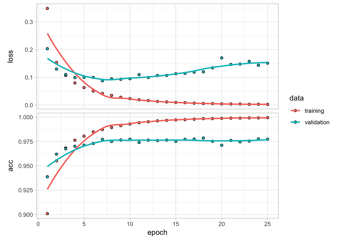

Figure 13.6: Training and validation performance over 25 epochs.

13.7 Model tuning

Now that we have an understanding of producing and running a DNN model, the next task is to find an optimal one by tuning different hyperparameters. There are many ways to tune a DNN. Typically, the tuning process follows these general steps; however, there is often a lot of iteration among these:

Adjust model capacity (layers & nodes);
Add batch normalization;
Add regularization;
Adjust learning rate.

13.7.1 Model capacity

Typically, we start by maximizing predictive performance based on model capacity. Higher model capacity (i.e., more layers and nodes) results in more memorization capacity for the model. On one hand, this can be good as it allows the model to learn more features and patterns in the data. On the other hand, a model with too much capacity will overfit to the training data. Typically, we look to maximize validation error performance while minimizing model capacity. As an example, we assessed nine different model capacity settings that include the following number of layers and nodes while maintaining all other parameters the same as the models in the previous sections (i.e.. our medium sized 2-hidden layer network contains 64 nodes in the first layer and 32 in the second.).

Table 13.1: Model capacities assessed represented as number of layers and nodes per layer.
	Hidden Layers
Size	1	2	3
small	16	16, 8	16, 8, 4
medium	64	64, 32	64, 32, 16
large	256	256, 128	256, 128, 64

The models that performed best had 2–3 hidden layers with a medium to large number of nodes. All the “small” models underfit and would require more epochs to identify their minimum validation error. The large 3-layer model overfits extremely fast. Preferably, we want a model that overfits more slowly such as the 1- and 2-layer medium and large models (Chollet and Allaire 2018).

If none of your models reach a flatlined validation error such as all the “small” models in Figure 13.7, increase the number of epochs trained. Alternatively, if your epochs flatline early then there is no reason to run so many epochs as you are just wasting computational energy with no gain. We can add a callback() function inside of fit() to help with this. There are multiple callbacks to help automate certain tasks. One such callback is early stopping, which will stop training if the loss function does not improve for a specified number of epochs.

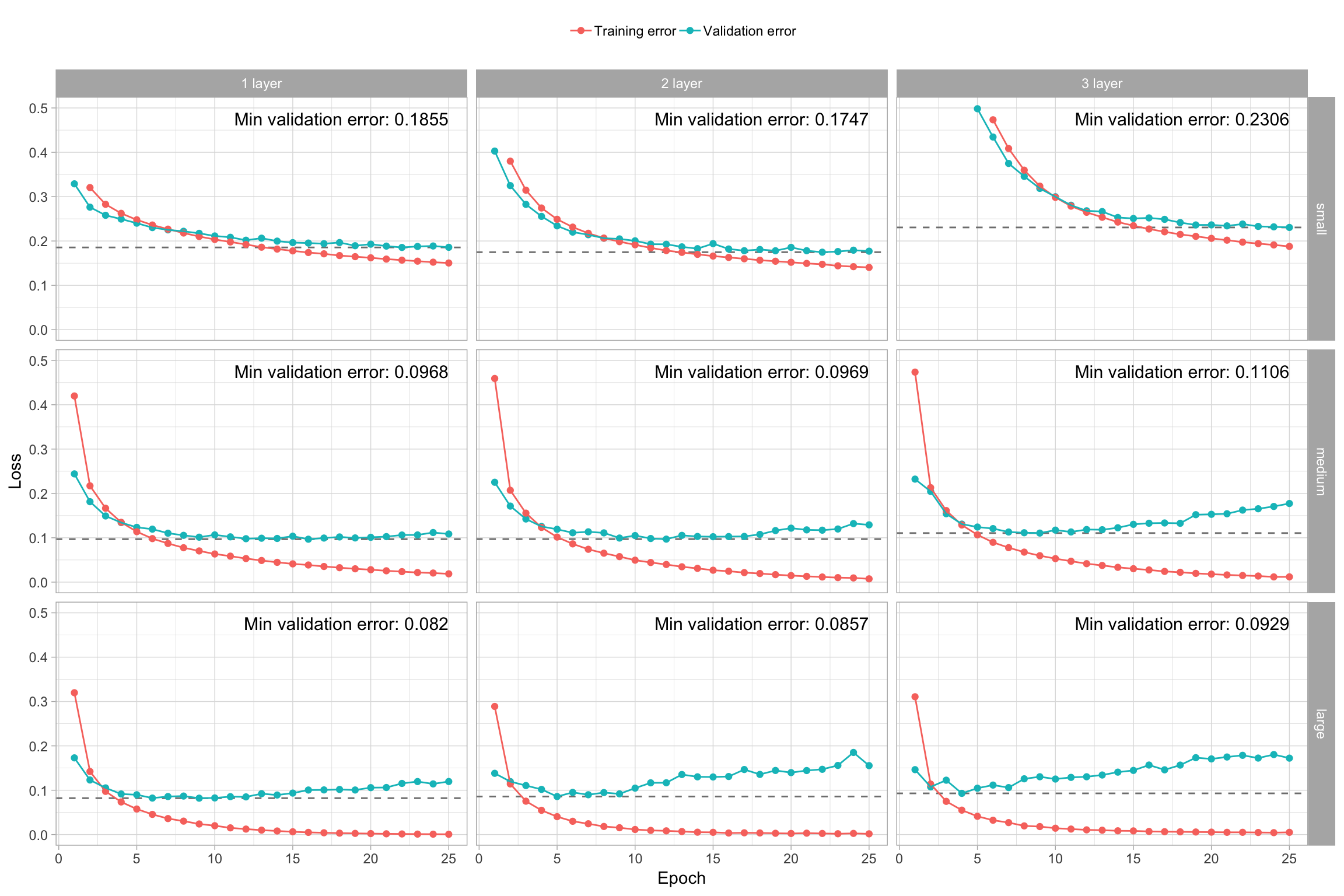
Figure 13.7: Training and validation performance for various model capacities.

13.7.2 Batch normalization

We’ve normalized the data before feeding it into our model, but data normalization should be a concern after every transformation performed by the network. Batch normalization (Ioffe and Szegedy 2015) is a recent advancement that adaptively normalizes data even as the mean and variance change over time during training. The main effect of batch normalization is that it helps with gradient propagation, which allows for deeper networks. Consequently, as the depth of your networks increase, batch normalization becomes more important and can improve performance.

We can add batch normalization by including layer_batch_normalization() after each middle layer within the network architecture section of our code:

model_w_norm <- keras_model_sequential() %>%
  
  # Network architecture with batch normalization
  layer_dense(units = 256, activation = "relu", input_shape = ncol(mnist_x)) %>%
  layer_batch_normalization() %>%
  layer_dense(units = 128, activation = "relu") %>%
  layer_batch_normalization() %>%
  layer_dense(units = 64, activation = "relu") %>%
  layer_batch_normalization() %>%
  layer_dense(units = 10, activation = "softmax") %>%

  # Backpropagation
  compile(
    loss = "categorical_crossentropy",
    optimizer = optimizer_rmsprop(),
    metrics = c("accuracy")
  )

If we add batch normalization to each of the previously assessed models, we see a couple patterns emerge. One, batch normalization often helps to minimize the validation loss sooner, which increases efficiency of model training. Two, we see that for the larger, more complex models (3-layer medium and 2- and 3-layer large), batch normalization helps to reduce the overall amount of overfitting. In fact, with batch normalization, our large 3-layer network now has the best validation error.

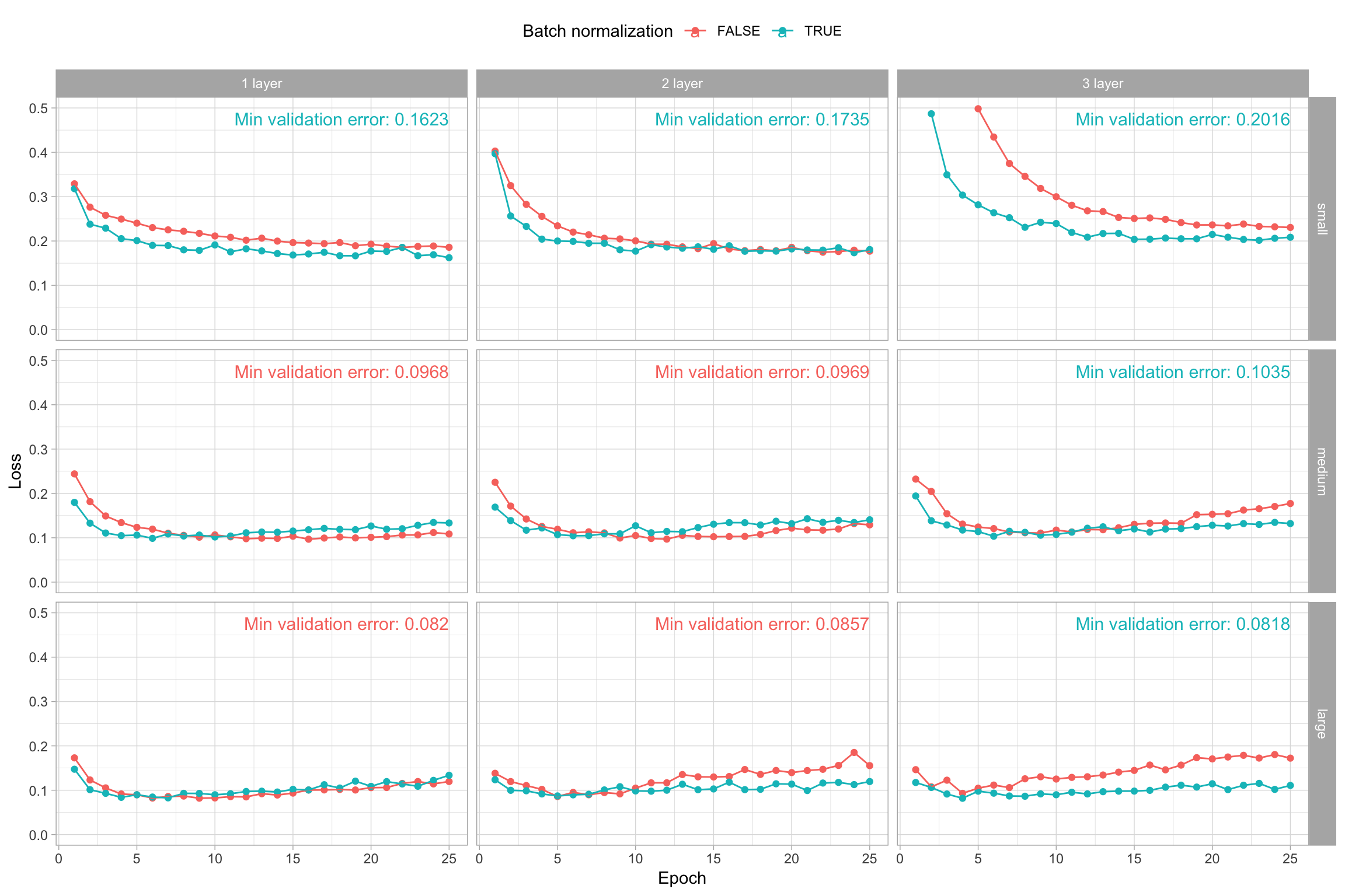
Figure 13.8: The effect of batch normalization on validation loss for various model capacities.

13.7.3 Regularization

As we’ve discussed in Chapters 6 and 12, placing constraints on a model’s complexity with regularization is a common way to mitigate overfitting. DNNs models are no different and there are two common approaches to regularizing neural networks. We can use an $L_1$ or $L_2$ penalty to add a cost to the size of the node weights, although the most common penalizer is the $L_2$ norm, which is called weight decay in the context of neural networks.³⁹ Regularizing the weights will force small signals (noise) to have weights nearly equal to zero and only allow consistently strong signals to have relatively larger weights.

As you add more layers and nodes, regularization with $L_1$ or $L_2$ penalties tend to have a larger impact on performance. Since having too many hidden units runs the risk of overparameterization, $L_1$ or $L_2$ penalties can shrink the extra weights toward zero to reduce the risk of overfitting.

We can add an $L_1$, $L_2$, or a combination of the two by adding regularizer_XX() within each layer.

model_w_reg <- keras_model_sequential() %>%
  
  # Network architecture with L1 regularization and batch normalization
  layer_dense(units = 256, activation = "relu", input_shape = ncol(mnist_x),
              kernel_regularizer = regularizer_l2(0.001)) %>%
  layer_batch_normalization() %>%
  layer_dense(units = 128, activation = "relu", 
              kernel_regularizer = regularizer_l2(0.001)) %>%
  layer_batch_normalization() %>%
  layer_dense(units = 64, activation = "relu", 
              kernel_regularizer = regularizer_l2(0.001)) %>%
  layer_batch_normalization() %>%
  layer_dense(units = 10, activation = "softmax") %>%

  # Backpropagation
  compile(
    loss = "categorical_crossentropy",
    optimizer = optimizer_rmsprop(),
    metrics = c("accuracy")
  )

Dropout (Srivastava et al. 2014 b; Hinton et al. 2012) is an additional regularization method that has become one of the most common and effectively used approaches to minimize overfitting in neural networks. Dropout in the context of neural networks randomly drops out (setting to zero) a number of output features in a layer during training. By randomly removing different nodes, we help prevent the model from latching onto happenstance patterns (noise) that are not significant. Typically, dropout rates range from 0.2–0.5 but can differ depending on the data (i.e., this is another tuning parameter). Similar to batch normalization, we can apply dropout by adding layer_dropout() in between the layers.

model_w_drop <- keras_model_sequential() %>%
  
  # Network architecture with 20% dropout
  layer_dense(units = 256, activation = "relu", input_shape = ncol(mnist_x)) %>%
  layer_dropout(rate = 0.2) %>%
  layer_dense(units = 128, activation = "relu") %>%
  layer_dropout(rate = 0.2) %>%
  layer_dense(units = 64, activation = "relu") %>%
  layer_dropout(rate = 0.2) %>%
  layer_dense(units = 10, activation = "softmax") %>%

  # Backpropagation
  compile(
    loss = "categorical_crossentropy",
    optimizer = optimizer_rmsprop(),
    metrics = c("accuracy")
  )

For our MNIST data, we find that adding an $L_1$ or $L_2$ cost does not improve our loss function. However, adding dropout does improve performance. For example, our large 3-layer model with 256, 128, and 64 nodes per respective layer so far has the best performance with a cross-entropy loss of 0.0818. However, as illustrated in Figure 13.8, this network still suffers from overfitting. Figure 13.9 illustrates the same 3-layer model with 256, 128, and 64 nodes per respective layers, batch normalization, and dropout rates of 0.4, 0.3, and 0.2 between each respective layer. We see a significant improvement in overfitting, which results in an improved loss score.

Note that as you constrain overfitting, often you need to increase the number of epochs to allow the network enough iterations to find the global minimal loss.

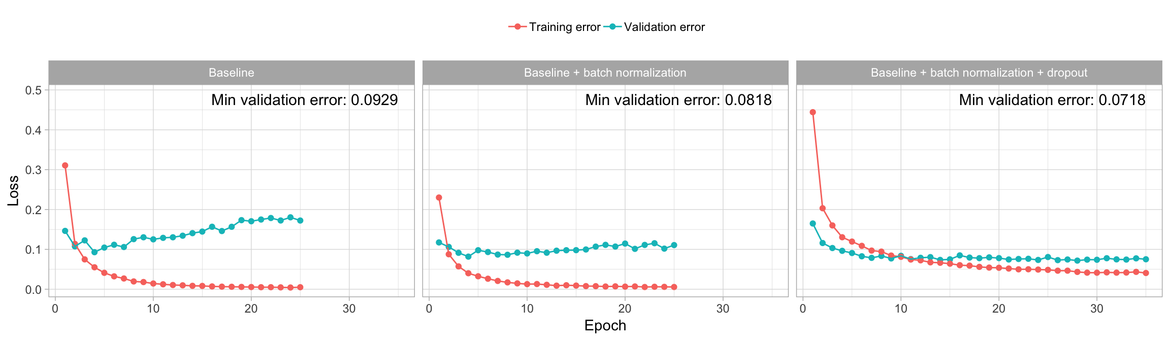
Figure 13.9: The effect of regularization with dropout on validation loss.

13.7.4 Adjust learning rate

Another issue to be concerned with is whether or not we are finding a global minimum versus a local minimum with our loss value. The mini-batch SGD optimizer we use will take incremental steps down our loss gradient until it no longer experiences improvement. The size of the incremental steps (i.e., the learning rate) will determine whether or not we get stuck in a local minimum instead of making our way to the global minimum.

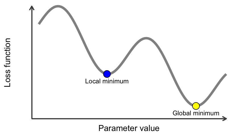
Figure 13.10: A local minimum and a global minimum.

There are two ways to circumvent this problem:

The different optimizers (e.g., RMSProp, Adam, Adagrad) have different algorithmic approaches for deciding the learning rate. We can adjust the learning rate of a given optimizer or we can adjust the optimizer used.
We can automatically adjust the learning rate by a factor of 2–10 once the validation loss has stopped improving.

The following builds onto our optimal model by changing the optimizer to Adam (Kingma and Ba 2014) and reducing the learning rate by a factor of 0.05 as our loss improvement begins to stall. We also add an early stopping argument to reduce unnecessary runtime. We see a slight improvement in performance and our loss curve in Figure 13.11 illustrates how we stop model training just as we begin to overfit.

model_w_adj_lrn <- keras_model_sequential() %>%
  layer_dense(units = 256, activation = "relu", input_shape = ncol(mnist_x)) %>%
  layer_batch_normalization() %>%
  layer_dropout(rate = 0.4) %>%
  layer_dense(units = 128, activation = "relu") %>%
  layer_batch_normalization() %>%
  layer_dropout(rate = 0.3) %>%
  layer_dense(units = 64, activation = "relu") %>%
  layer_batch_normalization() %>%
  layer_dropout(rate = 0.2) %>%
  layer_dense(units = 10, activation = "softmax") %>%
  compile(
    loss = 'categorical_crossentropy',
    optimizer = optimizer_adam(),
    metrics = c('accuracy')
  ) %>%
  fit(
    x = mnist_x,
    y = mnist_y,
    epochs = 35,
    batch_size = 128,
    validation_split = 0.2,
    callbacks = list(
      callback_early_stopping(patience = 5),
      callback_reduce_lr_on_plateau(factor = 0.05)
      ),
    verbose = FALSE
  )

model_w_adj_lrn
## Trained on 48,000 samples, validated on 12,000 samples (batch_size=128, epochs=20)
## Final epoch (plot to see history):
## val_loss: 0.07223
##  val_acc: 0.9808
##     loss: 0.05366
##      acc: 0.9832
##       lr: 0.001

# Optimal
min(model_w_adj_lrn$metrics$val_loss)
## [1] 0.0699492
max(model_w_adj_lrn$metrics$val_acc)
## [1] 0.981

# Learning rate
plot(model_w_adj_lrn)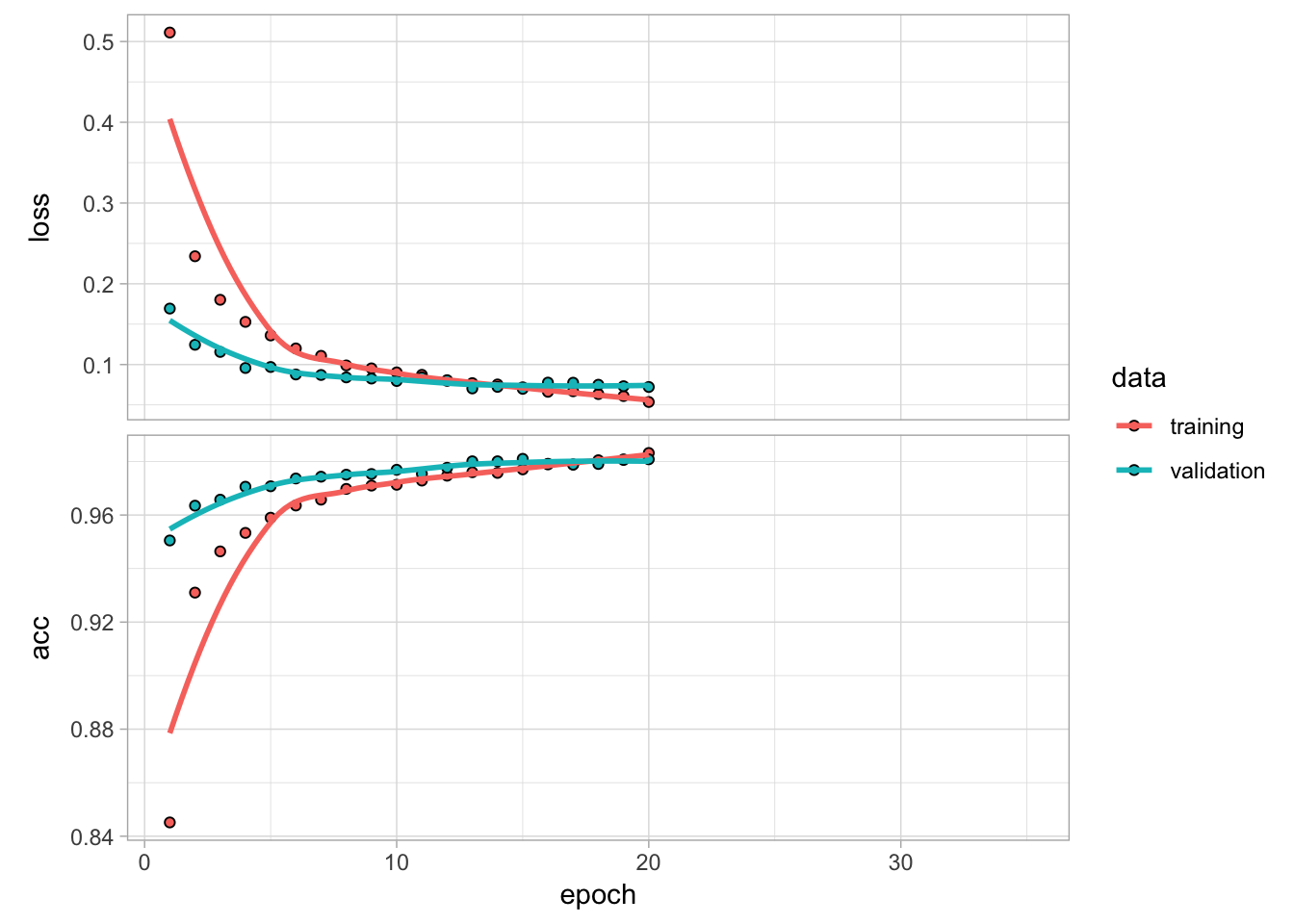

Training and validation performance on our 3-layer large network with dropout, adjustable learning rate, and using an Adam mini-batch SGD optimizer.

Figure 13.11: Training and validation performance on our 3-layer large network with dropout, adjustable learning rate, and using an Adam mini-batch SGD optimizer.

13.8 Grid Search

Hyperparameter tuning for DNNs tends to be a bit more involved than other ML models due to the number of hyperparameters that can/should be assessed and the dependencies between these parameters. For most implementations you need to predetermine the number of layers you want and then establish your search grid. If using h2o’s h2o.deeplearning() function, then creating and executing the search grid follows the same approach illustrated in Sections 11.5 and 12.4.2.

However, for keras, we use flags in a similar manner but their implementation provides added flexibility for tracking, visualizing, and managing training runs with the tfruns package (Allaire 2018). For a full discussion regarding flags see the https://tensorflow.rstudio.com/tools/ online resource. In this example we provide a training script mnist-grid-search.R that will be sourced for the grid search.

To create and perform a grid search, we first establish flags for the different hyperparameters of interest. These are considered the default flag values:

FLAGS <- flags(
  # Nodes
  flag_numeric("nodes1", 256),
  flag_numeric("nodes2", 128),
  flag_numeric("nodes3", 64),
  # Dropout
  flag_numeric("dropout1", 0.4),
  flag_numeric("dropout2", 0.3),
  flag_numeric("dropout3", 0.2),
  # Learning paramaters
  flag_string("optimizer", "rmsprop"),
  flag_numeric("lr_annealing", 0.1)
)

Next, we incorprate the flag parameters within our model:

model <- keras_model_sequential() %>%
  layer_dense(units = FLAGS$nodes1, activation = "relu", input_shape = ncol(mnist_x)) %>%
  layer_batch_normalization() %>%
  layer_dropout(rate = FLAGS$dropout1) %>%
  layer_dense(units = FLAGS$nodes2, activation = "relu") %>%
  layer_batch_normalization() %>%
  layer_dropout(rate = FLAGS$dropout2) %>%
  layer_dense(units = FLAGS$nodes3, activation = "relu") %>%
  layer_batch_normalization() %>%
  layer_dropout(rate = FLAGS$dropout3) %>%
  layer_dense(units = 10, activation = "softmax") %>%
  compile(
    loss = 'categorical_crossentropy',
    metrics = c('accuracy'),
    optimizer = FLAGS$optimizer
  ) %>%
  fit(
    x = mnist_x,
    y = mnist_y,
    epochs = 35,
    batch_size = 128,
    validation_split = 0.2,
    callbacks = list(
      callback_early_stopping(patience = 5),
      callback_reduce_lr_on_plateau(factor = FLAGS$lr_annealing)
    ),
    verbose = FALSE
  )

To execute the grid search we use tfruns::tuning_run(). Since our grid search assesses 2,916 combinations, we perform a random grid search and assess only 5% of the total models (sample = 0.05 which equates to 145 models). It becomes quite obvious that the hyperparameter search space explodes quickly with DNNs since there are so many model attributes that can be adjusted. Consequently, often a full Cartesian grid search is not possible due to time and computational constraints.

The optimal model has a validation loss of 0.0686 and validation accuracy rate of 0.9806 and the below code chunk shows the hyperparameter settings for this optimal model.

The following grid search took us over 1.5 hours to run!

# Run various combinations of dropout1 and dropout2
runs <- tuning_run("scripts/mnist-grid-search.R", 
  flags = list(
    nodes1 = c(64, 128, 256),
    nodes2 = c(64, 128, 256),
    nodes3 = c(64, 128, 256),
    dropout1 = c(0.2, 0.3, 0.4),
    dropout2 = c(0.2, 0.3, 0.4),
    dropout3 = c(0.2, 0.3, 0.4),
    optimizer = c("rmsprop", "adam"),
    lr_annealing = c(0.1, 0.05)
  ),
  sample = 0.05
)

runs %>% 
  filter(metric_val_loss == min(metric_val_loss)) %>% 
  glimpse()
## Observations: 1
## Variables: 31
## $ run_dir            <chr> "runs/2019-04-27T14-44-38Z"
## $ metric_loss        <dbl> 0.0598
## $ metric_acc         <dbl> 0.9806
## $ metric_val_loss    <dbl> 0.0686
## $ metric_val_acc     <dbl> 0.9806
## $ flag_nodes1        <int> 256
## $ flag_nodes2        <int> 128
## $ flag_nodes3        <int> 256
## $ flag_dropout1      <dbl> 0.4
## $ flag_dropout2      <dbl> 0.2
## $ flag_dropout3      <dbl> 0.3
## $ flag_optimizer     <chr> "adam"
## $ flag_lr_annealing  <dbl> 0.05
## $ samples            <int> 48000
## $ validation_samples <int> 12000
## $ batch_size         <int> 128
## $ epochs             <int> 35
## $ epochs_completed   <int> 17
## $ metrics            <chr> "runs/2019-04-27T14-44-38Z/tfruns.d/metrics.json"
## $ model              <chr> "Model\n_______________________________________________________…
## $ loss_function      <chr> "categorical_crossentropy"
## $ optimizer          <chr> "<tensorflow.python.keras.optimizers.Adam>"
## $ learning_rate      <dbl> 0.001
## $ script             <chr> "mnist-grid-search.R"
## $ start              <dttm> 2019-04-27 14:44:38
## $ end                <dttm> 2019-04-27 14:45:39
## $ completed          <lgl> TRUE
## $ output             <chr> "\n> #' Trains a feedforward DL model on the MNIST dataset.\n> …
## $ source_code        <chr> "runs/2019-04-27T14-44-38Z/tfruns.d/source.tar.gz"
## $ context            <chr> "local"
## $ type               <chr> "training"

13.9 Final thoughts

Training DNNs often requires more time and attention than other ML algorithms. With many other algorithms, the search space for finding an optimal model is small enough that Cartesian grid searches can be executed rather quickly. With DNNs, more thought, time, and experimentation is often required up front to establish a basic network architecture to build a grid search around. However, even with prior experimentation to reduce the scope of a grid search, the large number of hyperparameters still results in an exploding search space that can usually only be efficiently searched at random.

Historically, training neural networks was quite slow since runtime requires $O\left(NpML\right)$ operations where $N =$ # observations, $p=$ # features, $M=$ # hidden nodes, and $L=$ # epchos. Fortunately, software has advanced tremendously over the past decade to make execution fast and efficient. With open source software such as TensorFlow and Keras available via R APIs, performing state of the art deep learning methods is much more efficient, plus you get all the added benefits these open source tools provide (e.g., distributed computations across CPUs and GPUs, more advanced DNN architectures such as convolutional and recurrent neural nets, autoencoders, reinforcement learning, and more!).

References

Allaire, JJ. 2018. Tfruns: Training Run Tools for ’Tensorflow’. https://CRAN.R-project.org/package=tfruns.

Allaire, JJ, and François Chollet. 2019. Keras: R Interface to ’Keras’. https://keras.rstudio.com.

Chollet, François, and Joseph J Allaire. 2018. Deep Learning with R. Manning Publications Company.

Goodfellow, Ian, Yoshua Bengio, and Aaron Courville. 2016. Deep Learning. Vol. 1. MIT Press Cambridge.

Hinton, Geoffrey E, Nitish Srivastava, Alex Krizhevsky, Ilya Sutskever, and Ruslan R Salakhutdinov. 2012. “Improving Neural Networks by Preventing Co-Adaptation of Feature Detectors.” arXiv Preprint arXiv:1207.0580.

Ioffe, Sergey, and Christian Szegedy. 2015. “Batch Normalization: Accelerating Deep Network Training by Reducing Internal Covariate Shift.” arXiv Preprint arXiv:1502.03167.

Kingma, Diederik P, and Jimmy Ba. 2014. “Adam: A Method for Stochastic Optimization.” arXiv Preprint arXiv:1412.6980.

LeCun, Yann, Bernhard E Boser, John S Denker, Donnie Henderson, Richard E Howard, Wayne E Hubbard, and Lawrence D Jackel. 1990. “Handwritten Digit Recognition with a Back-Propagation Network.” In Advances in Neural Information Processing Systems, 396–404.

Ruder, Sebastian. 2016. “An Overview of Gradient Descent Optimization Algorithms.” arXiv Preprint arXiv:1609.04747.

Srivastava, Nitish, Geoffrey Hinton, Alex Krizhevsky, Ilya Sutskever, and Ruslan Salakhutdinov. 2014b. “Dropout: A Simple Way to Prevent Neural Networks from Overfitting.” The Journal of Machine Learning Research 15 (1). JMLR. org: 1929–58.

Not to be confused with shallow decision trees.↩
Standardization is not always necessary with neural networks. It largely depends on the type of network being trained. Feedforward networks, strictly speaking, do not require standardization; however, there are a variety of practical reasons why standardizing the inputs can make training faster and reduce the chances of getting stuck in local optima. Also, weight decay and Bayesian estimation can be applied more conveniently with standardized inputs (Sarle, Warren S., n.d.).↩
Often, the number of nodes in a layer is referred to as the network’s width while the number of layers in a model is referred to as its depth.↩
A gradient is the generalization of the concept of derivatives applied to functions of multidimensional inputs.↩
It’s considered stochastic because a random subset (batch) of observations is drawn for each forward pass.↩
Similar to the previous regularization discussions, the $L_1$ penalty is based on the absolute value of the weight coefficients, whereas the $L_2$ penalty is based on the square of the value of the weight coefficients.↩