Chapter 6 Regularized Regression

Linear models (LMs) provide a simple, yet effective, approach to predictive modeling. Moreover, when certain assumptions required by LMs are met (e.g., constant variance), the estimated coefficients are unbiased and, of all linear unbiased estimates, have the lowest variance. However, in today’s world, data sets being analyzed typically contain a large number of features. As the number of features grow, certain assumptions typically break down and these models tend to overfit the training data, causing our out of sample error to increase. Regularization methods provide a means to constrain or regularize the estimated coefficients, which can reduce the variance and decrease out of sample error.

6.1 Prerequisites

This chapter leverages the following packages. Most of these packages are playing a supporting role while the main emphasis will be on the glmnet package (Friedman et al. 2018).

# Helper packages
library(recipes)  # for feature engineering

# Modeling packages
library(glmnet)   # for implementing regularized regression
library(caret)    # for automating the tuning process

# Model interpretability packages
library(vip)      # for variable importance

To illustrate various regularization concepts we’ll continue working with the ames_train and ames_test data sets created in Section 2.7; however, at the end of the chapter we’ll also apply regularized regression to the employee attrition data.

6.2 Why regularize?

The easiest way to understand regularized regression is to explain how and why it is applied to ordinary least squares (OLS). The objective in OLS regression is to find the hyperplane²³ (e.g., a straight line in two dimensions) that minimizes the sum of squared errors (SSE) between the observed and predicted response values (see Figure 6.1 below). This means identifying the hyperplane that minimizes the grey lines, which measure the vertical distance between the observed (red dots) and predicted (blue line) response values.

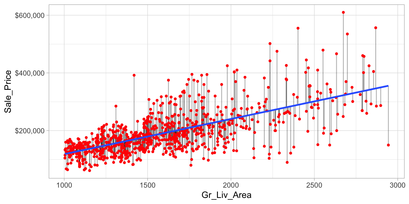
Figure 6.1: Fitted regression line using Ordinary Least Squares.

More formally, the objective function being minimized can be written as:

\[\begin{equation} \tag{6.1} \text{minimize} \left( SSE = \sum^n_{i=1} \left(y_i - \hat{y}_i\right)^2 \right) \end{equation}\]

As we discussed in Chapter 4, the OLS objective function performs quite well when our data adhere to a few key assumptions:

Linear relationship;
There are more observations (n) than features (p) ($n > p$);
No or little multicollinearity.

For classical statistical inference procedures (e.g., confidence intervals based on the classic t-statistic) to be valid, we also need to make stronger assumptions regarding normality (of the errors) and homoscedasticity (i.e., constant error variance).

Many real-life data sets, like those common to text mining and genomic studies are wide, meaning they contain a larger number of features ($p > n$). As p increases, we’re more likely to violate some of the OLS assumptions and alternative approaches should be considered. This was briefly illustrated in Chapter 4 where the presence of multicollinearity was diminishing the interpretability of our estimated coefficients due to inflated variance. By reducing multicollinearity, we were able to increase our model’s accuracy. Of course, multicollinearity can also occur when $n > p$.

Having a large number of features invites additional issues in using classic regression models. For one, having a large number of features makes the model much less interpretable. Additionally, when $p > n$, there are many (in fact infinite) solutions to the OLS problem! In such cases, it is useful (and practical) to assume that a smaller subset of the features exhibit the strongest effects (something called the bet on sparsity principle (see Hastie, Tibshirani, and Wainwright 2015, 2).). For this reason, we sometimes prefer estimation techniques that incorporate feature selection. One approach to this is called hard thresholding feature selection, which includes many of the traditional linear model selection approaches like forward selection and backward elimination. These procedures, however, can be computationally inefficient, do not scale well, and treat a feature as either in or out of the model (hence the name hard thresholding). In contrast, a more modern approach, called soft thresholding, slowly pushes the effects of irrelevant features toward zero, and in some cases, will zero out entire coefficients. As will be demonstrated, this can result in more accurate models that are also easier to interpret.

With wide data (or data that exhibits multicollinearity), one alternative to OLS regression is to use regularized regression (also commonly referred to as penalized models or shrinkage methods as in J. Friedman, Hastie, and Tibshirani (2001) and Kuhn and Johnson (2013)) to constrain the total size of all the coefficient estimates. This constraint helps to reduce the magnitude and fluctuations of the coefficients and will reduce the variance of our model (at the expense of no longer being unbiased—a reasonable compromise).

The objective function of a regularized regression model is similar to OLS, albeit with a penalty term $P$.

\[\begin{equation} \tag{6.2} \text{minimize} \left( SSE + P \right) \end{equation}\]

This penalty parameter constrains the size of the coefficients such that the only way the coefficients can increase is if we experience a comparable decrease in the sum of squared errors (SSE).

This concept generalizes to all GLM models (e.g., logistic and Poisson regression) and even some survival models. So far, we have been discussing OLS and the sum of squared errors loss function. However, different models within the GLM family have different loss functions (see Chapter 4 of J. Friedman, Hastie, and Tibshirani (2001)). Yet we can think of the penalty parameter all the same—it constrains the size of the coefficients such that the only way the coefficients can increase is if we experience a comparable decrease in the model’s loss function.

There are three common penalty parameters we can implement:

Ridge;
Lasso (or LASSO);
Elastic net (or ENET), which is a combination of ridge and lasso.

6.2.1 Ridge penalty

Ridge regression (Hoerl and Kennard 1970) controls the estimated coefficients by adding $\lambda \sum^p_{j=1} \beta_j^2$ to the objective function.

\[\begin{equation} \tag{6.3} \text{minimize } \left( SSE + \lambda \sum^p_{j=1} \beta_j^2 \right) \end{equation}\]

The size of this penalty, referred to as $L^2$ (or Euclidean) norm, can take on a wide range of values, which is controlled by the tuning parameter $\lambda$. When $\lambda = 0$ there is no effect and our objective function equals the normal OLS regression objective function of simply minimizing SSE. However, as $\lambda \rightarrow \infty$, the penalty becomes large and forces the coefficients toward zero (but not all the way). This is illustrated in Figure 6.2 where exemplar coefficients have been regularized with $\lambda$ ranging from 0 to over 8,000.

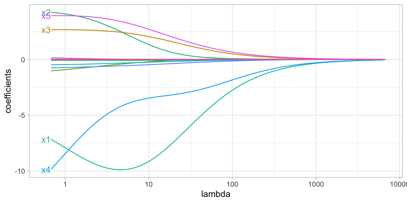
$Ridge regression coefficients for 15 exemplar predictor variables as $\lambda$ grows from $0 \rightarrow \infty$. As $\lambda$ grows larger, our coefficient magnitudes are more constrained.$

Figure 6.2: Ridge regression coefficients for 15 exemplar predictor variables as $\lambda$ grows from $0 \rightarrow \infty$. As $\lambda$ grows larger, our coefficient magnitudes are more constrained.

Although these coefficients were scaled and centered prior to the analysis, you will notice that some are quite large when $\lambda$ is near zero. Furthermore, you’ll notice that feature x1 has a large negative parameter that fluctuates until $\lambda \approx 7$ where it then continuously shrinks toward zero. This is indicative of multicollinearity and likely illustrates that constraining our coefficients with $\lambda > 7$ may reduce the variance, and therefore the error, in our predictions.

In essence, the ridge regression model pushes many of the correlated features toward each other rather than allowing for one to be wildly positive and the other wildly negative. In addition, many of the less-important features also get pushed toward zero. This helps to provide clarity in identifying the important signals in our data (i.e., the labeled features in Figure 6.2).

However, ridge regression does not perform feature selection and will retain all available features in the final model. Therefore, a ridge model is good if you believe there is a need to retain all features in your model yet reduce the noise that less influential variables may create (e.g., in smaller data sets with severe multicollinearity). If greater interpretation is necessary and many of the features are redundant or irrelevant then a lasso or elastic net penalty may be preferable.

6.2.2 Lasso penalty

The lasso (least absolute shrinkage and selection operator) penalty (Tibshirani 1996) is an alternative to the ridge penalty that requires only a small modification. The only difference is that we swap out the $L^2$ norm for an $L^1$ norm: $\lambda \sum^p_{j=1} | \beta_j|$:

\[\begin{equation} \tag{6.4} \text{minimize } \left( SSE + \lambda \sum^p_{j=1} | \beta_j | \right) \end{equation}\]

Whereas the ridge penalty pushes variables to approximately but not equal to zero, the lasso penalty will actually push coefficients all the way to zero as illustrated in Figure 6.3. Switching to the lasso penalty not only improves the model but it also conducts automated feature selection.

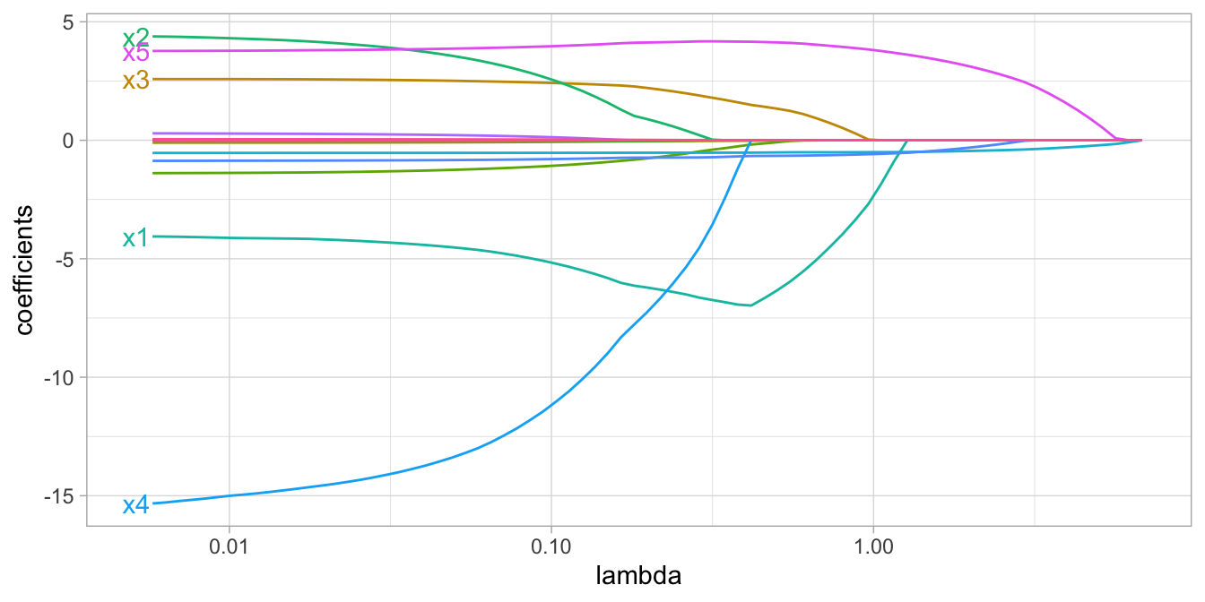
$Lasso regression coefficients as $\lambda$ grows from $0 \rightarrow \infty$.$

Figure 6.3: Lasso regression coefficients as $\lambda$ grows from $0 \rightarrow \infty$.

In the figure above we see that when $\lambda < 0.01$ all 15 variables are included in the model, when $\lambda \approx 0.5$ 9 variables are retained, and when $log\left(\lambda\right) = 1$ only 5 variables are retained. Consequently, when a data set has many features, lasso can be used to identify and extract those features with the largest (and most consistent) signal.

6.2.3 Elastic nets

A generalization of the ridge and lasso penalties, called the elastic net (Zou and Hastie 2005), combines the two penalties:

\[\begin{equation} \tag{6.5} \text{minimize } \left( SSE + \lambda_1 \sum^p_{j=1} \beta_j^2 + \lambda_2 \sum^p_{j=1} | \beta_j | \right) \end{equation}\]

Although lasso models perform feature selection, when two strongly correlated features are pushed towards zero, one may be pushed fully to zero while the other remains in the model. Furthermore, the process of one being in and one being out is not very systematic. In contrast, the ridge regression penalty is a little more effective in systematically handling correlated features together. Consequently, the advantage of the elastic net penalty is that it enables effective regularization via the ridge penalty with the feature selection characteristics of the lasso penalty.

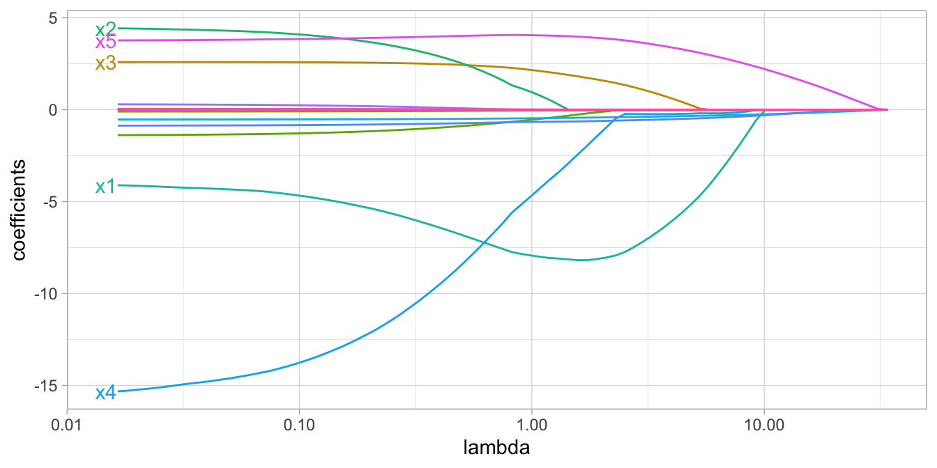
$Elastic net coefficients as $\lambda$ grows from $0 \rightarrow \infty$.$

Figure 6.4: Elastic net coefficients as $\lambda$ grows from $0 \rightarrow \infty$.

6.3 Implementation

First, we illustrate an implementation of regularized regression using the direct engine glmnet. This will provide you with a strong sense of what is happening with a regularized model. Realize there are other implementations available (e.g., h2o, elasticnet, penalized). Then, in Section 6.4, we’ll demonstrate how to apply a regularized model so we can properly compare it with our previous predictive models.

The glmnet package is extremely efficient and fast, even on very large data sets (mostly due to its use of Fortran to solve the lasso problem via coordinate descent); note, however, that it only accepts the non-formula XY interface (2.3.1) so prior to modeling we need to separate our feature and target sets.

The following uses model.matrix to dummy encode our feature set (see Matrix::sparse.model.matrix for increased efficiency on larger data sets). We also $\log$ transform the response variable which is not required; however, parametric models such as regularized regression are sensitive to skewed response values so transforming can often improve predictive performance.

# Create training  feature matrices
# we use model.matrix(...)[, -1] to discard the intercept
X <- model.matrix(Sale_Price ~ ., ames_train)[, -1]

# transform y with log transformation
Y <- log(ames_train$Sale_Price)

To apply a regularized model we can use the glmnet::glmnet() function. The alpha parameter tells glmnet to perform a ridge (alpha = 0), lasso (alpha = 1), or elastic net (0 < alpha < 1) model. By default, glmnet will do two things that you should be aware of:

Since regularized methods apply a penalty to the coefficients, we need to ensure our coefficients are on a common scale. If not, then predictors with naturally larger values (e.g., total square footage) will be penalized more than predictors with naturally smaller values (e.g., total number of rooms). By default, glmnet automatically standardizes your features. If you standardize your predictors prior to glmnet you can turn this argument off with standardize = FALSE.
glmnet will fit ridge models across a wide range of $\lambda$ values, which is illustrated in Figure 6.5.

# Apply ridge regression to ames data
ridge <- glmnet(
  x = X,
  y = Y,
  alpha = 0
)

plot(ridge, xvar = "lambda")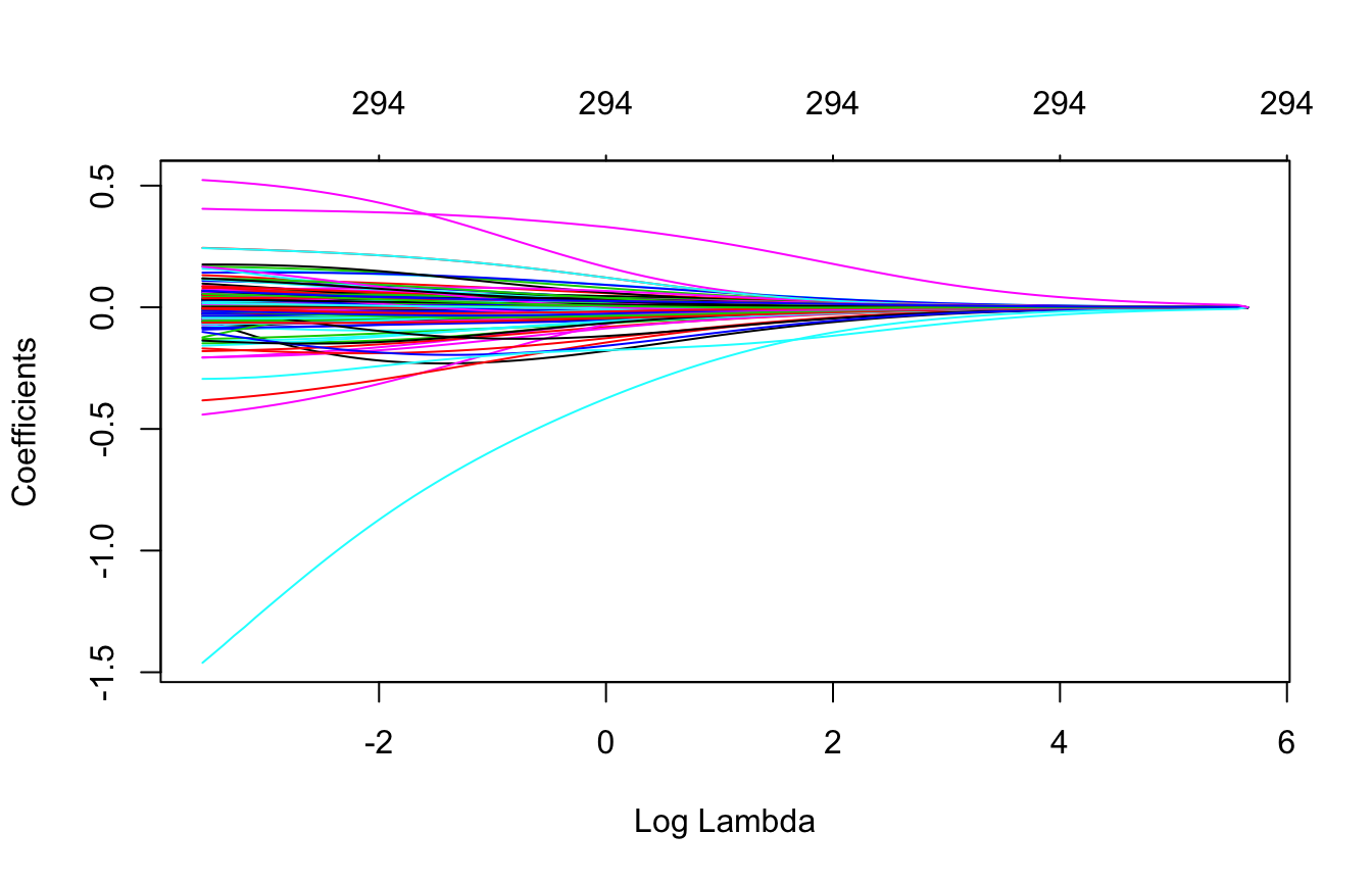

$Coefficients for our ridge regression model as $\lambda$ grows from $0 \rightarrow \infty$.$

Figure 6.5: Coefficients for our ridge regression model as $\lambda$ grows from $0 \rightarrow \infty$.

We can see the exact $\lambda$ values applied with ridge$lambda. Although you can specify your own $\lambda$ values, by default glmnet applies 100 $\lambda$ values that are data derived.

glmnet can auto-generate the appropriate $\lambda$ values based on the data; the vast majority of the time you will have little need to adjust this default.

We can also access the coefficients for a particular model using coef(). glmnet stores all the coefficients for each model in order of largest to smallest $\lambda$. Here we just peek at the two largest coefficients (which correspond to Latitude & Overall_QualVery_Excellent) for the largest (285.8054696) and smallest (0.0285805) $\lambda$ values. You can see how the largest $\lambda$ value has pushed most of these coefficients to nearly 0.

# lambdas applied to penalty parameter
ridge$lambda %>% head()
## [1] 285.8055 260.4153 237.2807 216.2014 196.9946 179.4942

# small lambda results in large coefficients
coef(ridge)[c("Latitude", "Overall_QualVery_Excellent"), 100]
##                   Latitude Overall_QualVery_Excellent 
##                  0.4048216                  0.1423770

# large lambda results in small coefficients
coef(ridge)[c("Latitude", "Overall_QualVery_Excellent"), 1]  
##                                      Latitude 
## 0.0000000000000000000000000000000000063823847 
##                    Overall_QualVery_Excellent 
## 0.0000000000000000000000000000000000009838114

At this point, we do not understand how much improvement we are experiencing in our loss function across various $\lambda$ values.

6.4 Tuning

Recall that $\lambda$ is a tuning parameter that helps to control our model from over-fitting to the training data. To identify the optimal $\lambda$ value we can use k-fold cross-validation (CV). glmnet::cv.glmnet() can perform k-fold CV, and by default, performs 10-fold CV. Below we perform a CV glmnet model with both a ridge and lasso penalty separately:

By default, glmnet::cv.glmnet() uses MSE as the loss function but you can also use mean absolute error (MAE) for continuous outcomes by changing the type.measure argument; see ?glmnet::cv.glmnet() for more details.

# Apply CV ridge regression to Ames data
ridge <- cv.glmnet(
  x = X,
  y = Y,
  alpha = 0
)

# Apply CV lasso regression to Ames data
lasso <- cv.glmnet(
  x = X,
  y = Y,
  alpha = 1
)

# plot results
par(mfrow = c(1, 2))
plot(ridge, main = "Ridge penalty\n\n")
plot(lasso, main = "Lasso penalty\n\n")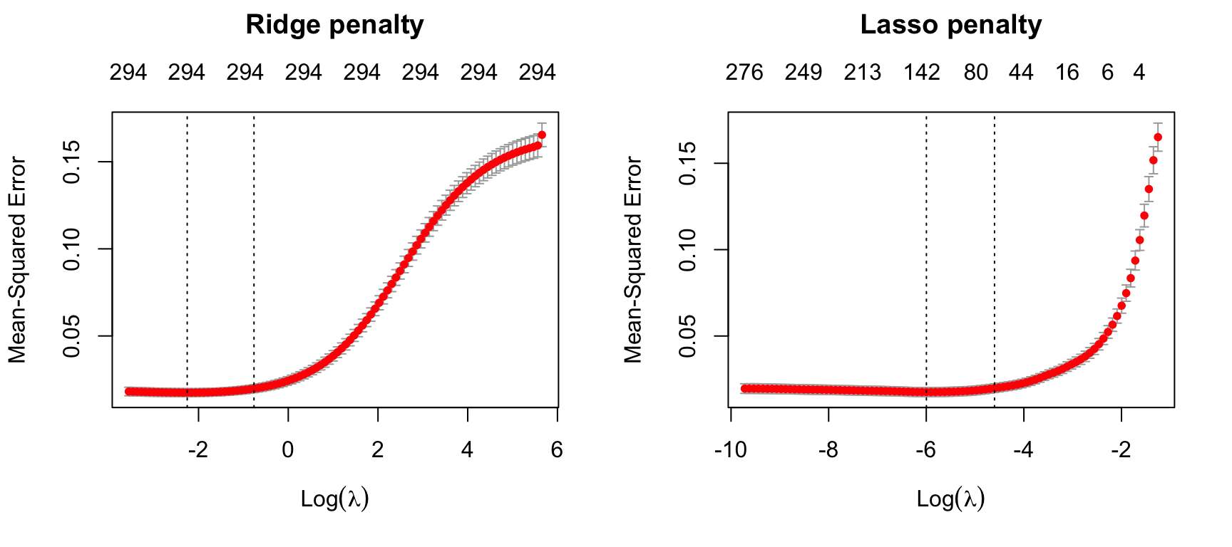

$10-fold CV MSE for a ridge and lasso model. First dotted vertical line in each plot represents the $\lambda$ with the smallest MSE and the second represents the $\lambda$ with an MSE within one standard error of the minimum MSE.$

Figure 6.6: 10-fold CV MSE for a ridge and lasso model. First dotted vertical line in each plot represents the $\lambda$ with the smallest MSE and the second represents the $\lambda$ with an MSE within one standard error of the minimum MSE.

Figure 6.6 illustrates the 10-fold CV MSE across all the $\lambda$ values. In both models we see a slight improvement in the MSE as our penalty $log(\lambda)$ gets larger, suggesting that a regular OLS model likely overfits the training data. But as we constrain it further (i.e., continue to increase the penalty), our MSE starts to increase. The numbers across the top of the plot refer to the number of features in the model. Ridge regression does not force any variables to exactly zero so all features will remain in the model but we see the number of variables retained in the lasso model decrease as the penalty increases.

The first and second vertical dashed lines represent the $\lambda$ value with the minimum MSE and the largest $\lambda$ value within one standard error of it. The minimum MSE for our ridge model is 0.01748 (produced when $\lambda =$ 0.10513 whereas the minimum MSE for our lasso model is 0.01754 (produced when $\lambda =$ 0.00249).

# Ridge model
min(ridge$cvm)       # minimum MSE
## [1] 0.01748122
ridge$lambda.min     # lambda for this min MSE
## [1] 0.1051301

ridge$cvm[ridge$lambda == ridge$lambda.1se]  # 1-SE rule
## [1] 0.01975572
ridge$lambda.1se  # lambda for this MSE
## [1] 0.4657917

# Lasso model
min(lasso$cvm)       # minimum MSE
## [1] 0.01754244
lasso$lambda.min     # lambda for this min MSE
## [1] 0.00248579
lasso$nzero[lasso$lambda == lasso$lambda.min] # No. of coef | Min MSE
## s51 
## 139

lasso$cvm[lasso$lambda == lasso$lambda.1se]  # 1-SE rule
## [1] 0.01979976
lasso$lambda.1se  # lambda for this MSE
## [1] 0.01003518
lasso$nzero[lasso$lambda == lasso$lambda.1se] # No. of coef | 1-SE MSE
## s36 
##  64

We can assess this visually. Figure 6.7 plots the estimated coefficients across the range of $\lambda$ values. The dashed red line represents the $\lambda$ value with the smallest MSE and the dashed blue line represents largest $\lambda$ value that falls within one standard error of the minimum MSE. This shows you how much we can constrain the coefficients while still maximizing predictive accuracy.

Above, we saw that both ridge and lasso penalties provide similar MSEs; however, these plots illustrate that ridge is still using all 294 features whereas the lasso model can get a similar MSE while reducing the feature set from 294 down to 139. However, there will be some variability with this MSE and we can reasonably assume that we can achieve a similar MSE with a slightly more constrained model that uses only 64 features. Although this lasso model does not offer significant improvement over the ridge model, we get approximately the same accuracy by using only 64 features! If describing and interpreting the predictors is an important component of your analysis, this may significantly aid your endeavor.

# Ridge model
ridge_min <- glmnet(
  x = X,
  y = Y,
  alpha = 0
)

# Lasso model
lasso_min <- glmnet(
  x = X,
  y = Y,
  alpha = 1
)

par(mfrow = c(1, 2))
# plot ridge model
plot(ridge_min, xvar = "lambda", main = "Ridge penalty\n\n")
abline(v = log(ridge$lambda.min), col = "red", lty = "dashed")
abline(v = log(ridge$lambda.1se), col = "blue", lty = "dashed")

# plot lasso model
plot(lasso_min, xvar = "lambda", main = "Lasso penalty\n\n")
abline(v = log(lasso$lambda.min), col = "red", lty = "dashed")
abline(v = log(lasso$lambda.1se), col = "blue", lty = "dashed")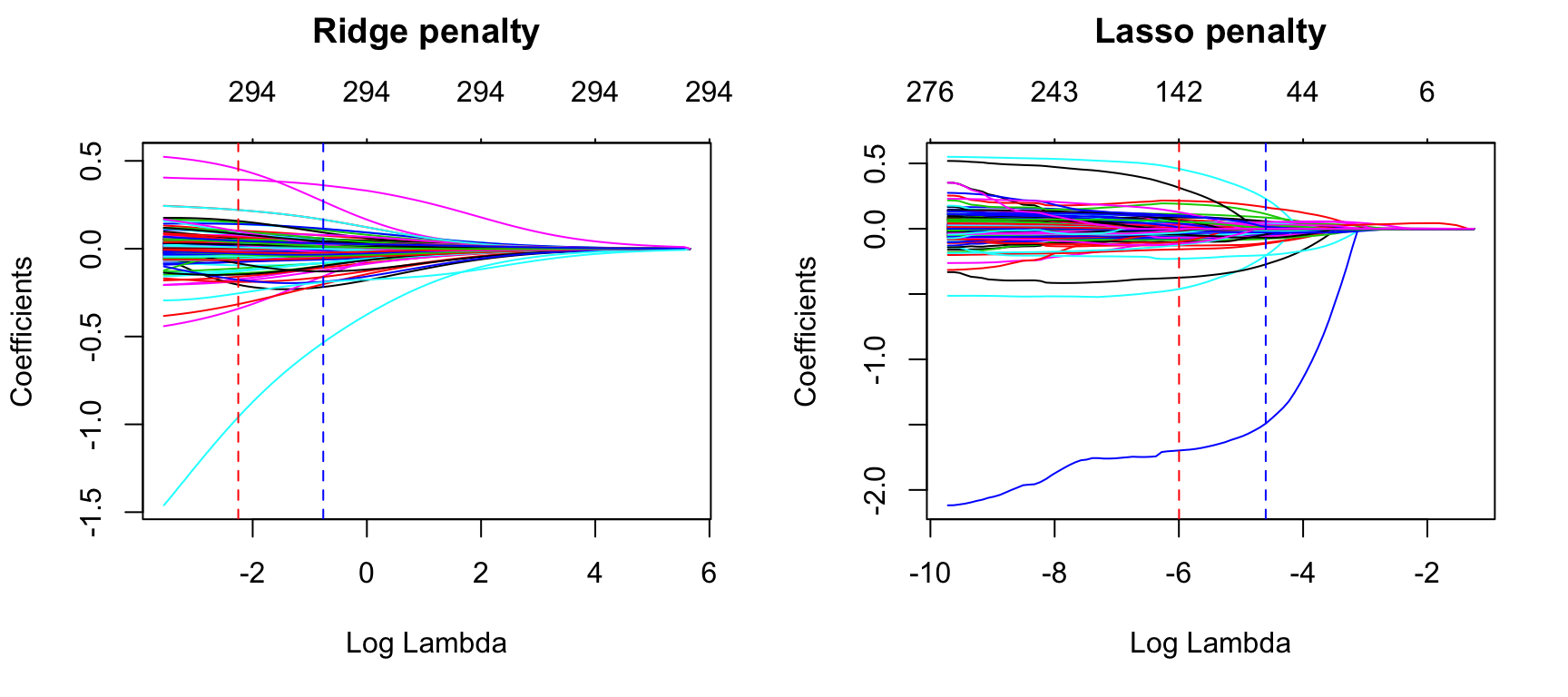

$Coefficients for our ridge and lasso models. First dotted vertical line in each plot represents the $\lambda$ with the smallest MSE and the second represents the $\lambda$ with an MSE within one standard error of the minimum MSE.$

Figure 6.7: Coefficients for our ridge and lasso models. First dotted vertical line in each plot represents the $\lambda$ with the smallest MSE and the second represents the $\lambda$ with an MSE within one standard error of the minimum MSE.

So far we’ve implemented a pure ridge and pure lasso model. However, we can implement an elastic net the same way as the ridge and lasso models, by adjusting the alpha parameter. Any alpha value between 0–1 will perform an elastic net. When alpha = 0.5 we perform an equal combination of penalties whereas alpha $< 0.5$ will have a heavier ridge penalty applied and alpha $> 0.5$ will have a heavier lasso penalty.

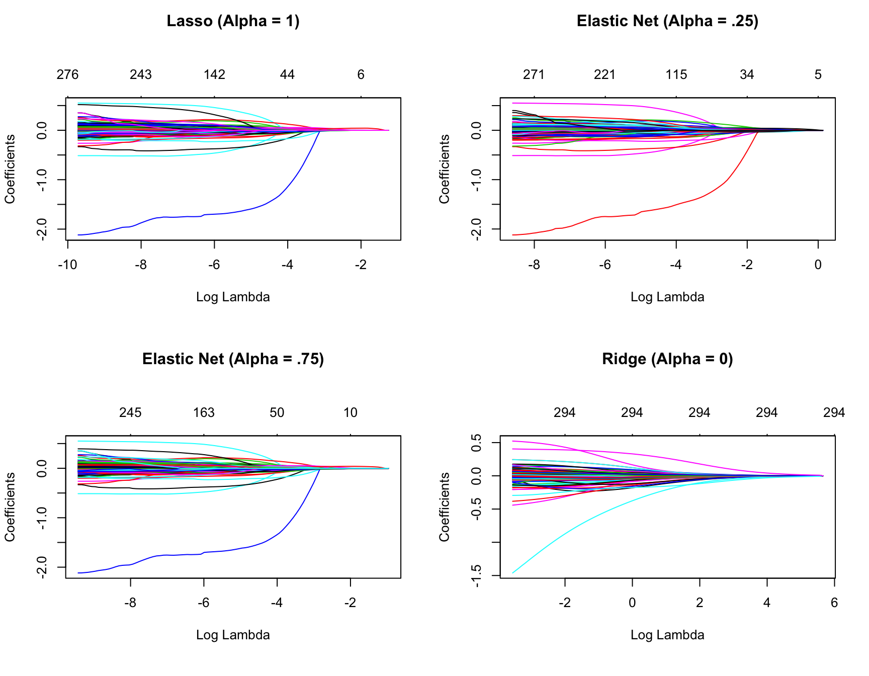
Figure 6.8: Coefficients for various penalty parameters.

Often, the optimal model contains an alpha somewhere between 0–1, thus we want to tune both the $\lambda$ and the alpha parameters. As in Chapters 4 and 5, we can use the caret package to automate the tuning process. This ensures that any feature engineering is appropriately applied within each resample. The following performs a grid search over 10 values of the alpha parameter between 0–1 and ten values of the lambda parameter from the lowest to highest lambda values identified by glmnet.

This grid search took roughly 71 seconds to compute.

The following snippet of code shows that the model that minimized RMSE used an alpha of 0.1 and $\lambda$ of 0.02. The minimum RMSE of 0.1277585 ($MSE = 0.1277585^2 = 0.01632223$) slightly improves upon the full ridge and lasso models produced earlier. Figure 6.9 illustrates how the combination of alpha values ($x$-axis) and $\lambda$ values (line color) influence the RMSE.

# for reproducibility
set.seed(123)

# grid search across 
cv_glmnet <- train(
  x = X,
  y = Y,
  method = "glmnet",
  preProc = c("zv", "center", "scale"),
  trControl = trainControl(method = "cv", number = 10),
  tuneLength = 10
)

# model with lowest RMSE
cv_glmnet$bestTune
##   alpha     lambda
## 7   0.1 0.02007035

# results for model with lowest RMSE
cv_glmnet$results %>%
  filter(alpha == cv_glmnet$bestTune$alpha, lambda == cv_glmnet$bestTune$lambda)
##   alpha     lambda      RMSE  Rsquared        MAE     RMSESD RsquaredSD
## 1   0.1 0.02007035 0.1277585 0.9001487 0.08102427 0.02235901  0.0346677
##         MAESD
## 1 0.005667366

# plot cross-validated RMSE
ggplot(cv_glmnet)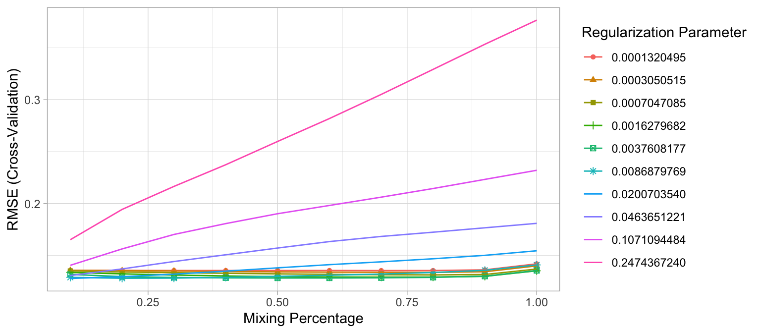

Figure 6.9: The 10-fold cross valdation RMSE across 10 alpha values (x-axis) and 10 lambda values (line color).

So how does this compare to our previous best model for the Ames data set? Keep in mind that for this chapter we $\log$ transformed the response variable (Sale_Price). Consequently, to provide a fair comparison to our previously obtained PLS model’s RMSE of $25,460, we need to re-transform our predicted values. The following illustrates that our optimal regularized model achieved an RMSE of $19,905. Introducing a penalty parameter to constrain the coefficients provided quite an improvement over our previously obtained dimension reduction approach.

# predict sales price on training data
pred <- predict(cv_glmnet, X)

# compute RMSE of transformed predicted
RMSE(exp(pred), exp(Y))
## [1] 19905.05

6.5 Feature interpretation

Variable importance for regularized models provides a similar interpretation as in linear (or logistic) regression. Importance is determined by magnitude of the standardized coefficients and we can see in Figure 6.10 some of the same features that were considered highly influential in our PLS model, albeit in differing order (i.e. Gr_Liv_Area, Total_Bsmt_SF, Overall_Qual, Year_Built).

vip(cv_glmnet, num_features = 20, geom = "point")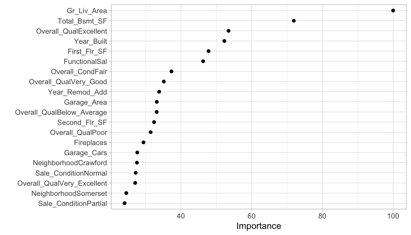

Figure 6.10: Top 20 most important variables for the optimal regularized regression model.

Similar to linear and logistic regression, the relationship between the features and response is monotonic linear. However, since we modeled our response with a log transformation, the estimated relationships will still be monotonic but non-linear on the original response scale. Figure 6.11 illustrates the relationship between the top four most influential variables (i.e., largest absolute coefficients) and the non-transformed sales price. All relationships are positive in nature, as the values in these features increase (or for Overall_QualExcellent if it exists) the average predicted sales price increases.

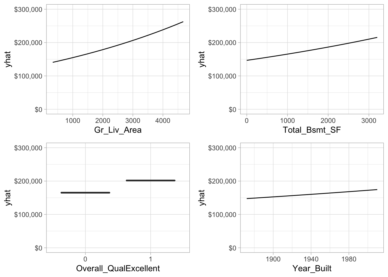
Figure 6.11: Partial dependence plots for the first four most important variables.

However, not that one of the top 20 most influential variables is Overall_QualPoor. When a home has an overall quality rating of poor we see that the average predicted sales price decreases versus when it has some other overall quality rating. Consequently, its important to not only look at the variable importance ranking, but also observe the positive or negative nature of the relationship.

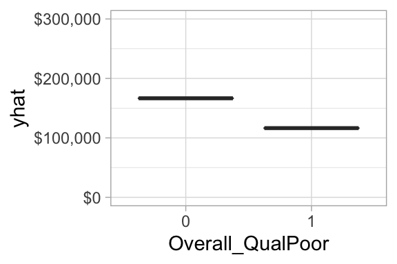
Figure 6.12: Partial dependence plot for when overall quality of a home is (1) versus is not poor (0).

6.6 Attrition data

We saw that regularization significantly improved our predictive accuracy for the Ames data set, but how about for the employee attrition example? In Chapter 5 we saw a maximum CV accuracy of 86.3% for our logistic regression model. We see a little improvement in the following with some preprocessing; however, performing a regularized logistic regression model provides us with an additional 0.8% improvement in accuracy (likely within the margin of error).

df <- attrition %>% mutate_if(is.ordered, factor, ordered = FALSE)

# Create training (70%) and test (30%) sets for the
# rsample::attrition data. Use set.seed for reproducibility
set.seed(123)
churn_split <- initial_split(df, prop = .7, strata = "Attrition")
train <- training(churn_split)
test  <- testing(churn_split)

# train logistic regression model
set.seed(123)
glm_mod <- train(
  Attrition ~ ., 
  data = train, 
  method = "glm",
  family = "binomial",
  preProc = c("zv", "center", "scale"),
  trControl = trainControl(method = "cv", number = 10)
  )

# train regularized logistic regression model
set.seed(123)
penalized_mod <- train(
  Attrition ~ ., 
  data = train, 
  method = "glmnet",
  family = "binomial",
  preProc = c("zv", "center", "scale"),
  trControl = trainControl(method = "cv", number = 10),
  tuneLength = 10
  )

# extract out of sample performance measures
summary(resamples(list(
  logistic_model = glm_mod, 
  penalized_model = penalized_mod
  )))$statistics$Accuracy
##                      Min.   1st Qu.    Median      Mean   3rd Qu.
## logistic_model  0.8365385 0.8495146 0.8792476 0.8757893 0.8907767
## penalized_model 0.8446602 0.8759280 0.8834951 0.8835759 0.8915469
##                      Max. NA's
## logistic_model  0.9313725    0
## penalized_model 0.9411765    0

6.7 Final thoughts

Regularized regression provides many great benefits over traditional GLMs when applied to large data sets with lots of features. It provides a great option for handling the $n > p$ problem, helps minimize the impact of multicollinearity, and can perform automated feature selection. It also has relatively few hyperparameters which makes them easy to tune, computationally efficient compared to other algorithms discussed in later chapters, and memory efficient.

However, regularized regression does require some feature preprocessing. Notably, all inputs must be numeric; however, some packages (e.g., caret and h2o) automate this process. They cannot automatically handle missing data, which requires you to remove or impute them prior to modeling. Similar to GLMs, they are also not robust to outliers in both the feature and target. Lastly, regularized regression models still assume a monotonic linear relationship (always increasing or decreasing in a linear fashion). It is also up to the analyst whether or not to include specific interaction effects.

References

Friedman, Jerome, Trevor Hastie, and Robert Tibshirani. 2001. The Elements of Statistical Learning. Vol. 1. Springer Series in Statistics New York, NY, USA:

Friedman, Jerome, Trevor Hastie, Rob Tibshirani, Noah Simon, Balasubramanian Narasimhan, and Junyang Qian. 2018. Glmnet: Lasso and Elastic-Net Regularized Generalized Linear Models. https://CRAN.R-project.org/package=glmnet.

Hastie, T., R. Tibshirani, and M. Wainwright. 2015. Statistical Learning with Sparsity: The Lasso and Generalizations. Chapman & Hall/Crc Monographs on Statistics & Applied Probability. Taylor & Francis.

Hoerl, Arthur E, and Robert W Kennard. 1970. “Ridge Regression: Biased Estimation for Nonorthogonal Problems.” Technometrics 12 (1). Taylor & Francis Group: 55–67.

Kuhn, Max, and Kjell Johnson. 2013. Applied Predictive Modeling. Vol. 26. Springer.

Tibshirani, Robert. 1996. “Regression Shrinkage and Selection via the Lasso.” Journal of the Royal Statistical Society. Series B (Methodological). JSTOR, 267–88.

Zou, Hui, and Trevor Hastie. 2005. “Regularization and Variable Selection via the Elastic Net.” Journal of the Royal Statistical Society: Series B (Statistical Methodology) 67 (2). Wiley Online Library: 301–20.

See Section 14.2 for more discussion on hyperplanes.↩