Chapter 14 Support Vector Machines

Support vector machines (SVMs) offer a direct approach to binary classification: try to find a hyperplane in some feature space that “best” separates the two classes. In practice, however, it is difficult (if not impossible) to find a hyperplane to perfectly separate the classes using just the original features. SVMs overcome this by extending the idea of finding a separating hyperplane in two ways: (1) loosen what we mean by “perfectly separates”, and (2) use the so-called kernel trick to enlarge the feature space to the point that perfect separation of classes is (more) likely.

14.1 Prerequisites

Although there are a number of great packages that implement SVMs (e.g., e1071 (Meyer et al. 2019) and svmpath (Hastie 2016)), we’ll focus on the most flexible implementation of SVMs in R: kernlab (Karatzoglou et al. 2004). We’ll also use caret for tuning SVMs and pre-processing. In this chapter, we’ll explicitly load the following packages:

# Helper packages
library(dplyr)    # for data wrangling
library(ggplot2)  # for awesome graphics
library(rsample)  # for data splitting

# Modeling packages
library(caret)    # for classification and regression training
library(kernlab)  # for fitting SVMs

# Model interpretability packages
library(pdp)      # for partial dependence plots, etc.
library(vip)      # for variable importance plots

To illustrate the basic concepts of fitting SVMs we’ll use a mix of simulated data sets as well as the employee attrition data. The code for generating the simulated data sets and figures in this chapter are available on the book website. In the employee attrition example our intent is to predict on Attrition (coded as "Yes"/"No"). As in previous chapters, we’ll set aside 30% of the data for assessing generalizability.

# Load attrition data
df <- attrition %>% 
  mutate_if(is.ordered, factor, ordered = FALSE)

# Create training (70%) and test (30%) sets
set.seed(123)  # for reproducibility
churn_split <- initial_split(df, prop = 0.7, strata = "Attrition")
churn_train <- training(churn_split)
churn_test  <- testing(churn_split)

14.2 Optimal separating hyperplanes

Rather than diving right into SVMs we’ll build up to them using concepts from basic geometry, starting with hyperplanes. A hyperplane in \(p\)-dimensional feature space is defined by the (linear) equation

\[f\left(X\right) = \beta_0 + \beta_1 X_1 + \dots + \beta_p X_p = 0\]

When \(p = 2\), this defines a line in 2-D space, and when \(p = 3\), it defines a plane in 3-D space (see Figure 14.1). By definition, for points on one side of the hyperplane, \(f\left(X\right) > 0\), and for points on the other side, \(f\left(X\right) < 0\). For (mathematical) convenience, we’ll re-encode the binary outcome \(Y_i\) using {-1, 1} so that \(Y_i \times f\left(X_i\right) > 0\) for points on the correct side of the hyperplane. In this context the hyperplane represents a decision boundary that partitions the feature space into two sets, one for each class. The SVM will classify all the points on one side of the decision boundary as belonging to one class and all those on the other side as belonging to the other class.

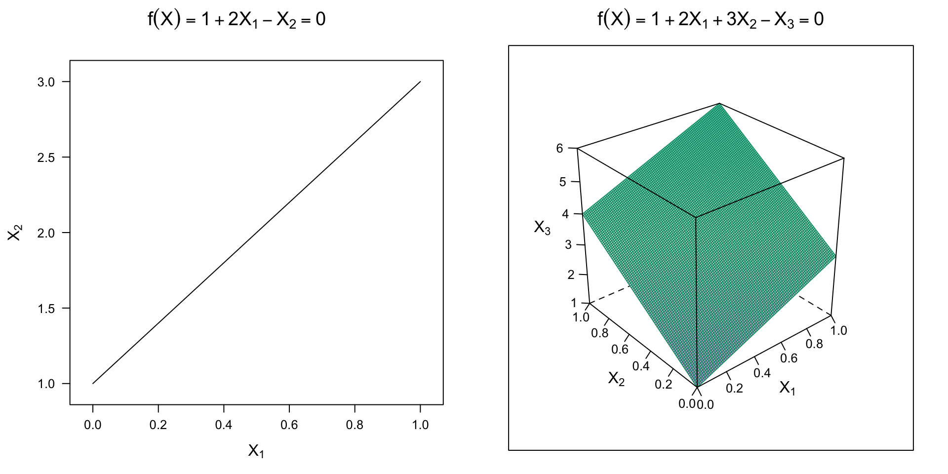
Figure 14.1: Examples of hyperplanes in 2-D and 3-D feature space.

While SVMs may seem mathematically frightening at first, the fundamental ideas behind them are incredibly intuitive and easy to understand. We’ll illustrate these simple ideas using simulated binary classification data with two features. In this hypothetical example, we have two classes: households that own a riding lawn mower (\(Y = +1\)) and (2) households that do not (\(Y = -1\)). We also have two features, household income (\(X_1\)) and lot size (\(X_2\)), that have been standardized (i.e., centered around zero with a standard deviation of one). Intuitively, we might expect households with a larger lot and a higher income to be more likely to own a riding mower. In fact, the two classes in the left side of Figure 14.2 are perfectly separable by a straight line (i.e., a hyperplane in 2-D space).

14.2.1 The hard margin classifier

As you might imagine, for two separable classes, there are an infinite number of separating hyperplanes! This is illustrated in the right side of Figure 14.2 where we show the hyperplanes (i.e., decision boundaries) that result from a simple logistic regression model (GLM), a linear discriminant analysis (LDA; another popular classification tool), and an example of a hard margin classifier (HMC)—which we’ll define in a moment. So which decision boundary is “best”? Well, it depends on how we define “best”. If you were asked to draw a decision boundary with good generalization performance on the left side of Figure 14.2, how would it look to you? Naturally, you would probably draw a boundary that provides the maximum separation between the two classes, and that’s exactly what the HMC is doing!

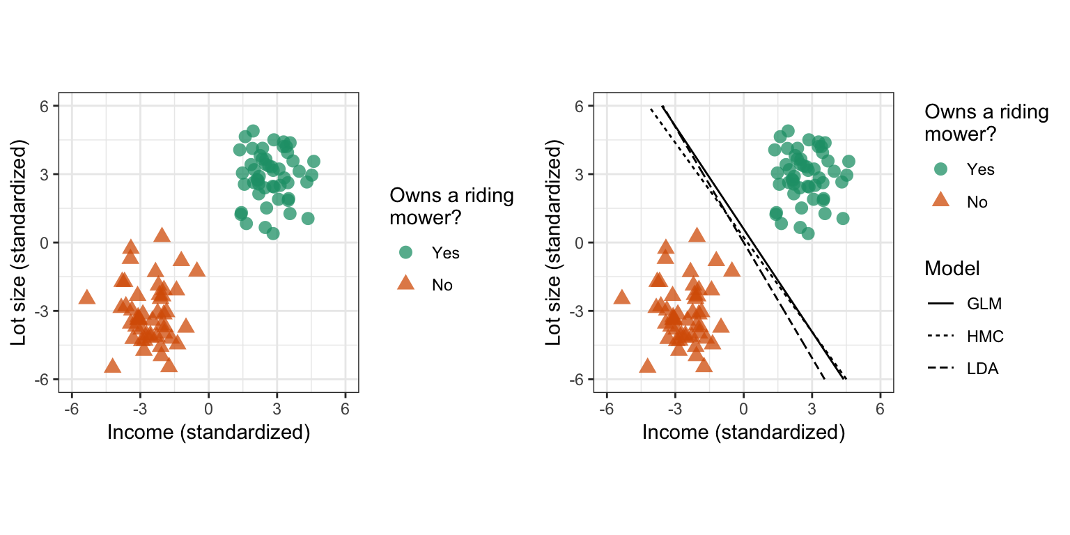
Figure 14.2: Simulated binary classification data with two separable classes. Left: Raw data. Right: Raw data with example decision boundaries (in this case, separating hyperplanes) from various machine learning algorithms.

Although we can draw an unlimited number of separating hyperplanes, what we want is a separating hyperplane with good generalization performance! The HMC is one such “optimal” separating hyperplane and the simplest type of SVM. The HMC is optimal in the sense that it separates the two classes while maximizing the distance to the closest points from either class; see Figure 14.3 below. The decision boundary (i.e., hyperplane) from the HMC separates the two classes by maximizing the distance between them. This maximized distance is referred to as the margin \(M\) (the shaded areas in Figure 14.3). Finding this decision boundary can also be done with simple geometry. Geometrically, finding the HMC for two separable classes amounts to the following:

1. Draw the convex hull⁴⁰ around each class (these are the polygons surrounding each class in Figure 14.3).

2. Draw the shortest line segment that connects the two convex hulls (this is the dotted line segment in Figure 14.3).

3. The perpendicular bisector of this line segment is the HMC!

4. The margin boundaries are formed by drawing lines that pass through the support vectors and are parallel to the separating hyperplane (these are the dashed line segments in Figure 14.3).

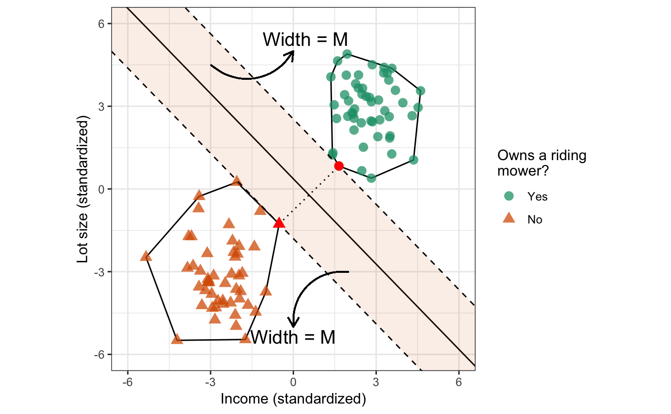
Figure 14.3: HMC for the simulated riding mower data. The solid black line forms the decision boundary (in this case, a separating hyperplane), while the dashed lines form the boundaries of the margins (shaded regions) on each side of the hyperplane. The shortest distance between the two classes (i.e., the dotted line connecting the two convex hulls) has length \(2M\). Two of the training observations (solid red points) fall on the margin boundaries; in the context of SVMs (which we discuss later), these two points form the support vectors.

This can also be formulated as an optimization problem. Mathematically speaking, the HMC estimates the coefficients of the hyperplane by solving a quadratic programming problem with linear inequality constraints, in particular:

\[\begin{align} &\underset{\beta_0, \beta_1, \dots, \beta_p}{\text{maximize}} \quad M \\ &\text{subject to} \quad \begin{cases} \sum_{j = 1}^p \beta_j^2 = 1,\\ y_i\left(\beta_0 + \beta_1 x_{i1} + \dots + \beta_p x_{ip}\right) \ge M,\quad i = 1, 2, \dots, n \end{cases} \end{align}\]

Put differently, the HMC finds the separating hyperplane that provides the largest margin/gap between the two classes. The width of both margin boundaries is \(M\). With the constraint \(\sum_{j = 1}^p \beta_j^2 = 1\), the quantity \(y_i\left(\beta_0 + \beta_1 x_{i1} + \dots + \beta_p x_{ip}\right)\) represents the distance from the \(i\)-th data point to the decision boundary. Note that the solution to the optimization problem above does not allow any points to be on the wrong side of the margin; hence the term hard margin classifier.

14.2.2 The soft margin classifier

Sometimes perfect separation is achievable, but not desirable! Take, for example, the data in Figure 14.4. Here we added a single outlier at the point \(\left(0.5, 1\right)\). While the data are still perfectly separable, the decision boundaries obtained using logistic regression and the HMC will not generalize well to new data and accuracy will suffer (i.e., these models are not robust to outliers in the feature space). The LDA model seems to produce a more reasonable decision boundary.

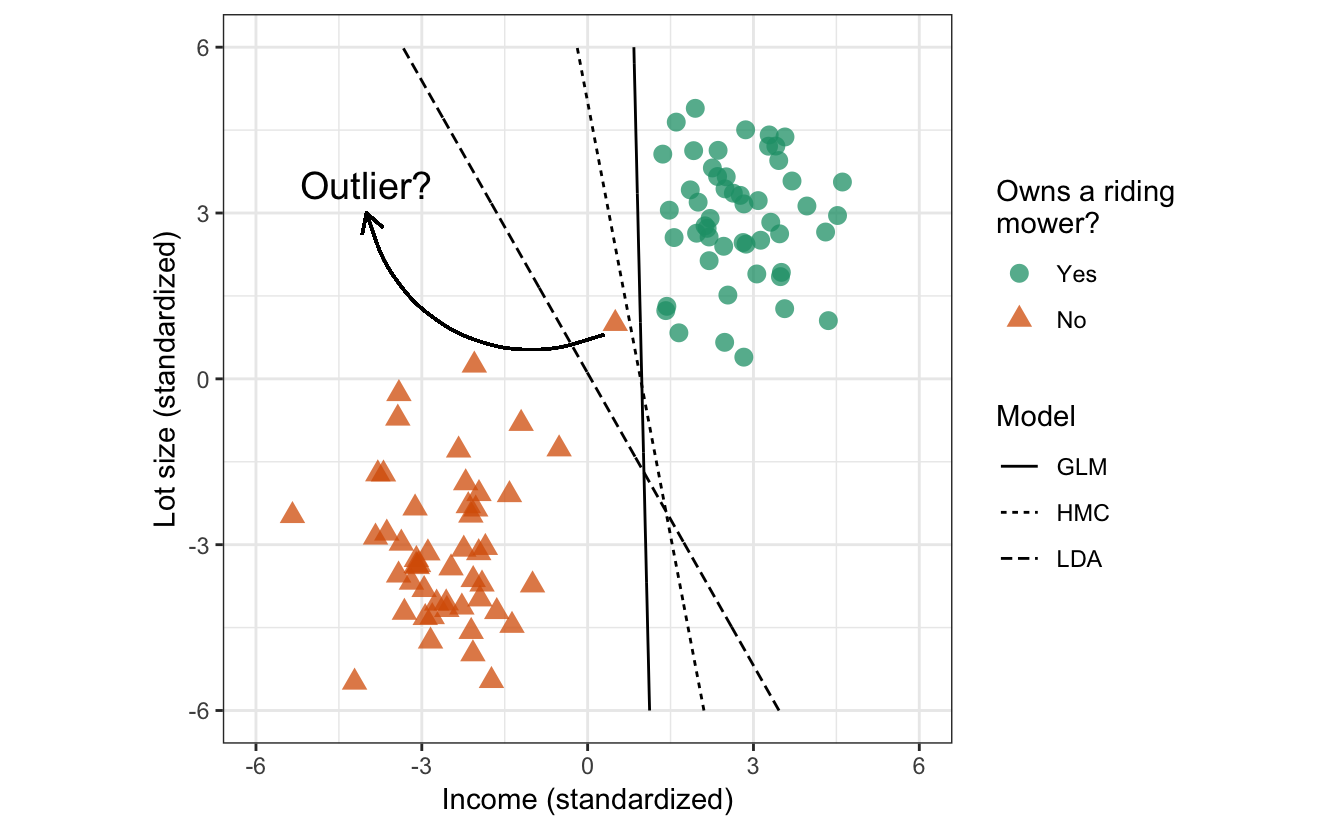
Figure 14.4: Simulated binary classification data with an outlier at the point \(\left(0.5, 1\right)\).

In this situation, we can loosen the constraints (or soften the margin) by allowing some points to be on the wrong side of the margin; this is referred to as the the soft margin classifier (SMC). The SMC, similar to the HMC, estimates the coefficients of the hyperplane by solving the slightly modified optimization problem:

\[\begin{align} &\underset{\beta_0, \beta_1, \dots, \beta_p}{\text{maximize}} \quad M \\ &\text{subject to} \quad \begin{cases} \sum_{j = 1}^p \beta_j^2 = 1,\\ y_i\left(\beta_0 + \beta_1 x_{i1} + \dots + \beta_p x_{ip}\right) \ge M\left(1 - \xi_i\right), \quad i = 1, 2, \dots, n\\ \xi_i \ge 0, \\ \sum_{i = 1}^n \xi_i \le C\end{cases} \end{align}\]

Similar to before, the SMC finds the separating hyperplane that provides the largest margin/gap between the two classes, but allows for some of the points to cross over the margin boundaries. Here \(C\) is the allowable budget for the total amount of overlap and is our first tunable hyperparameter for the SVM.

By varying \(C\), we allow points to violate the margin which helps make the SVM robust to outliers. For example, in Figure 14.5, we fit the SMC at both extremes: \(C = 0\) (the HMC) and \(C = \infty\) (maximum overlap). Ideally, the hyperplane giving the decision boundary with the best generalization performance lies somewhere in between these two extremes and can be determined using, for example, k-fold CV.

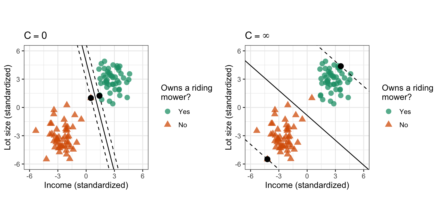
Figure 14.5: Soft margin classifier. Left: Zero budget for overlap (i.e., the HMC). Right: Maximumn allowable overlap. The solid black points represent the support vectors that define the margin boundaries.

14.3 The support vector machine

So far, we’ve only used linear decision boundaries. Such a classifier is likely too restrictive to be useful in practice, especially when compared to other algorithms that can adapt to nonlinear relationships. Fortunately, we can use a simple trick, called the kernel trick, to overcome this. A deep understanding of the kernel trick requires an understanding of kernel functions and reproducing kernel Hilbert spaces 😱. Fortunately, we can use a couple illustrations in 2-D/3-D feature space to drive home the key idea.

Consider, for example, the circle data on the left side of Figure 14.6. This is another binary classification problem. The first class forms a circle in the middle of a square, the remaining points form the second class. Although these two classes do not overlap (although they appear to overlap slightly due to the size of the plotted points), they are not perfectly separable by a hyperplane (i.e., a straight line). However, we can enlarge the feature space by adding a third feature, say \(X_3 = X_1^2 + X_2^2\)—this is akin to using the polynomial kernel function discussed below with \(d = 2\). The data are plotted in the enlarged feature space in the middle of Figure 14.6. In this new three dimensional feature space, the two classes are perfectly separable by a hyperplane (i.e., a flat plane); though it is hard to see (see the middle of Figure 14.6), the green points form the tip of the hyperboloid in 3-D feature space (i.e., \(X_3\) is smaller for all the green points leaving a small gap between the two classes). The resulting decision boundary is then projected back onto the original feature space resulting in a non-linear decision boundary which perfectly separates the original data (see the right side of Figure 14.6)!

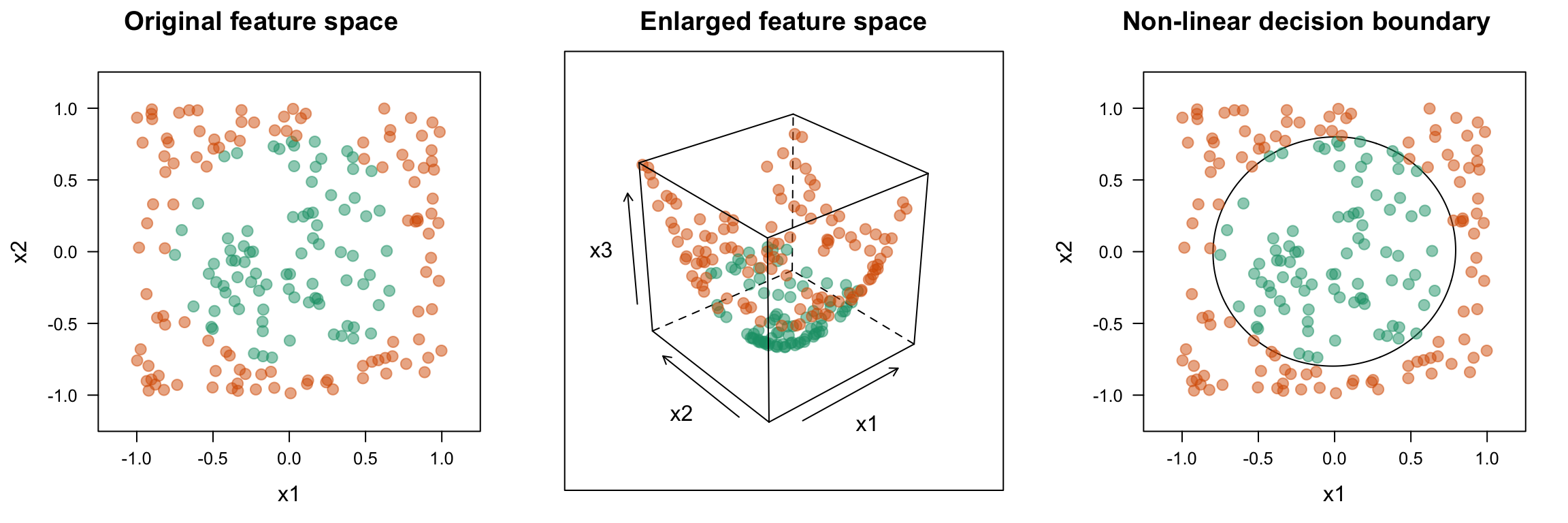
Figure 14.6: Simulated nested circle data. Left: The two classes in the original (2-D) feature space. Middle: The two classes in the enlarged (3-D) feature space. Right: The decision boundary from the HMC in the enlarged feature space projected back into the original feature space.

In essence, SVMs use the kernel trick to enlarge the feature space using basis functions (e.g., like in MARS or polynomial regression). In this enlarged (kernel-induced) feature space, a hyperplane can often separate the two classes. The resulting decision boundary, which is linear in the enlarged feature space, will be nonlinear when transformed back onto the original feature space.

Popular kernel functions used by SVMs include:

• d-th degree polynomial: \(K\left(x, x'\right) = \gamma\left(1 + \langle x, x' \rangle\right) ^ d\)

• Radial basis function: \(K\left(x, x'\right) = \exp\left(\gamma \lVert x - x'\rVert ^ 2\right)\)

• Hyperbolic tangent: \(K\left(x, x'\right) = \tanh\left(k_1\lVert x - x'\rVert + k_2\right)\)

Here \(\langle x, x' \rangle = \sum_{i = 1}^n x_i x_i'\) is called an inner product. Notice how each of these kernel functions include hyperparameters that need to be tuned. For example, the polynomial kernel includes a degree term \(d\) and a scale parameter \(\gamma\). Similarly, the radial basis kernel includes a \(\gamma\) parameter related to the inverse of the \(\sigma\) parameter of a normal distribution. In R, you can use caret’s getModelInfo() to extract the hyperparameters from various SVM implementations with different kernel functions, for example:

# Linear (i.e., soft margin classifier)
caret::getModelInfo("svmLinear")$svmLinear$parameters
##   parameter   class label
## 1         C numeric  Cost

# Polynomial kernel
caret::getModelInfo("svmPoly")$svmPoly$parameters
##   parameter   class             label
## 1    degree numeric Polynomial Degree
## 2     scale numeric             Scale
## 3         C numeric              Cost

# Radial basis kernel
caret::getModelInfo("svmRadial")$svmRadial$parameters
##   parameter   class label
## 1     sigma numeric Sigma
## 2         C numeric  Cost

Through the use of various kernel functions, SVMs are extremely flexible and capable of estimating complex nonlinear decision boundaries. For example, the right side of Figure 14.7 demonstrates the flexibility of an SVM using a radial basis kernel applied to the two spirals benchmark problem (see ?mlbench::mlbench.spirals for details). As a reference, the left side of Figure 14.7 shows the decision boundary from a default random forest fit using the ranger package. The random forest decision boundary, while flexible, has trouble capturing smooth decision boundaries (like a spiral). The SVM with a radial basis kernel, on the other hand, does a great job (and in this case is more accurate).

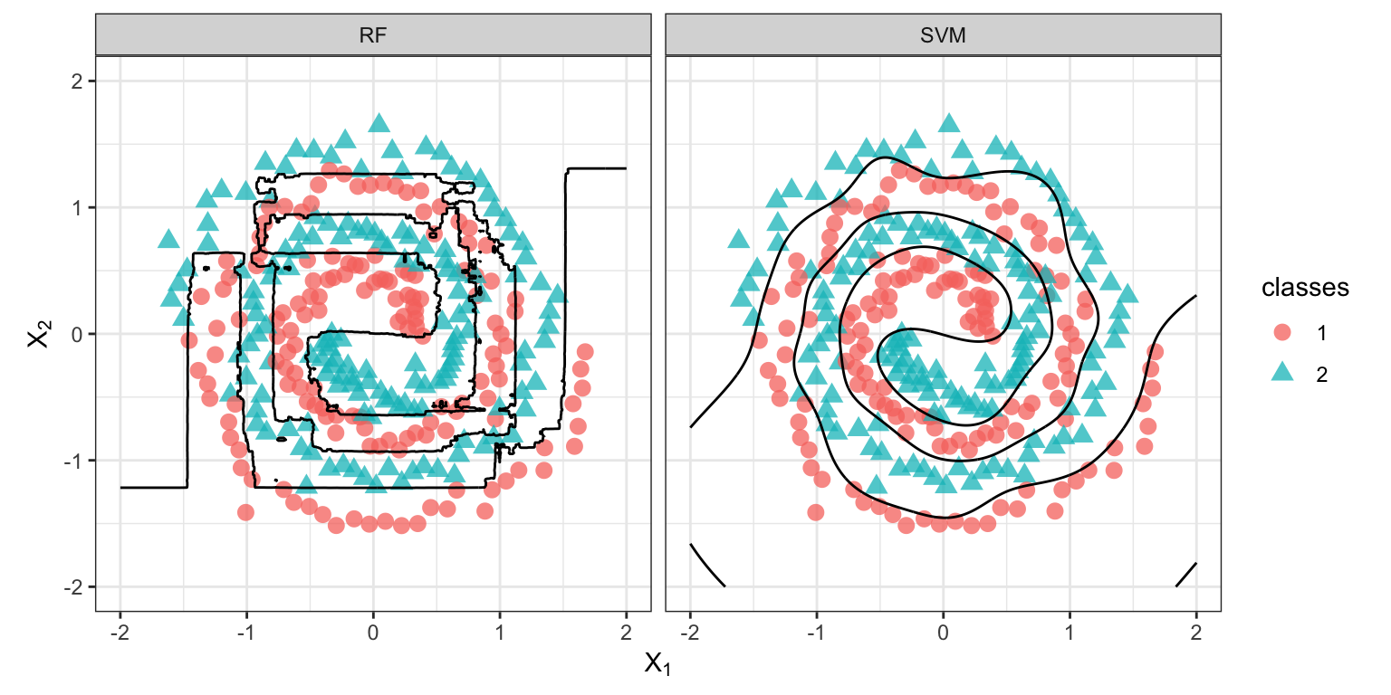
Figure 14.7: Two spirals benchmark problem. Left: Decision boundary from a random forest. Right: Decision boundary from an SVM with radial basis kernel.

The radial basis kernel is extremely flexible and as a rule of thumb, we generally start with this kernel when fitting SVMs in practice.

14.3.1 More than two classes

The SVM, as introduced, is applicable to only two classes! What do we do when we have more than two classes? There are two general approaches: one-versus-all (OVA) and one-versus-one (OVO). In OVA, we fit an SVM for each class (one class versus the rest) and classify to the class for which the margin is the largest. In OVO, we fit all \(\binom{\# \ classes}{2}\) pairwise SVMs and classify to the class that wins the most pairwise competitions. All the popular implementations of SVMs, including kernlab, provide such approaches to multinomial classification.

14.3.2 Support vector regression

SVMs can also be extended to regression problems (i.e., when the outcome is continuous). In essence, SVMs find a separating hyperplane in an enlarged feature space that generally results in a nonlinear decision boundary in the original feature space with good generalization performance. This enlarged feature spaced is constructed using special functions called kernel functions. The idea behind support vector regression (SVR) is very similar: find a good fitting hyperplane in a kernel-induced feature space that will have good generalization performance using the original features. Although there are many flavors of SVR, we’ll introduce the most common: \(\epsilon\)-insensitive loss regression.

Recall that the least squares (LS) approach to function estimation (Chapter 4) minimizes the sum of the squared residuals, where in general we define the residual as \(r\left(x, y\right) = y - f\left(x\right)\). (In ordinary linear regression \(f\left(x\right) = \beta_0 + \beta_1 x_1 + \dots + \beta_p x_p\)). The problem with LS is that it involves squaring the residuals which gives outliers undue influence on the fitted regression function. Although we could rely on the MAE metric (which looks at the absolute value as opposed to the squared residuals), another intuitive loss metric, called \(\epsilon\)-insensitive loss, is more robust to outliers:

\[ L_{\epsilon} = max\left(0, \left|r\left(x, y\right)\right| - \epsilon\right) \]

Here \(\epsilon\) is a threshold set by the analyst. In essence, we’re forming a margin around the regression curve of width \(\epsilon\) (see Figure 14.8), and trying to contain as many data points within the margin as possible with a minimal number of violations. The data points that satisfy \(r\left(x, y\right) \pm \epsilon\) form the support vectors that define the margin. The model is said to be \(\epsilon\)-insensitive because the points within the margin have no influence on the fitted regression line! Similar to SVMs, we can use kernel functions to capture nonlinear relationships (in this case, the support vectors are those points who’s residuals satisfy \(r\left(x, y\right) \pm \epsilon\) in the kernel-induced feature space).

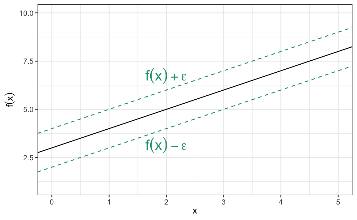
Figure 14.8: \(\epsilon\)-insensitive regression band. The solid black line represents the estimated regression curve \(f\left(x\right)\).

To illustrate, we simulated data from the sinc function \(\sin\left(x\right) / x\) with added Gaussian nose (i.e., random errors from a normal distribution). The simulated data are shown in Figure 14.9. This is a highly nonlinear, but smooth function of \(x\).

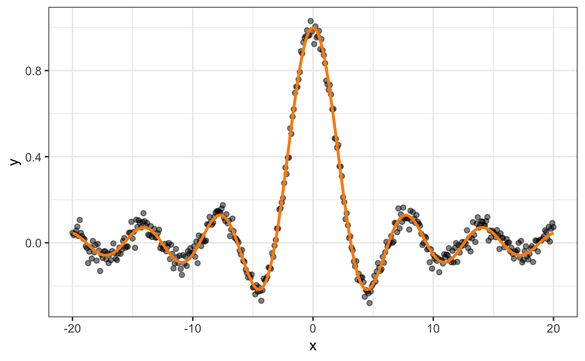
Figure 14.9: Simulated data from a sinc function with added noise.

We fit three regression models to these data: a default MARS model (Chapter 7), a default RF (Chapter 11), and an SVR model using \(\epsilon\)-insensitive loss and a radial basis kernel with default tuning parameters (technically, we set kpar = "automatic" which tells kernlab::ksvm() to use kernlab::sigest() to find a reasonable estimate for the kernel’s scale parameter). To use \(\epsilon\)-insensitive loss regression, specify type = "eps-svr" in the call to kernlab::ksvm() (the default for \(\epsilon\) is epsilon = 0.1. The results are displayed in Figure 14.10. Although this is a simple one-dimensional problem, the MARS and RF struggle to adapt to the smooth, but highly nonlinear function. The MARS model, while probably effective, is too rigid and fails to adequately capture the relationship towards the left-hand side. The RF is too wiggly and is indicative of slight overfitting (perhaps tuning the minimum observations per node can help here and is left as an exercise on the book website). The SVR model, on the other hand, works quite well and provides a smooth fit to the data!

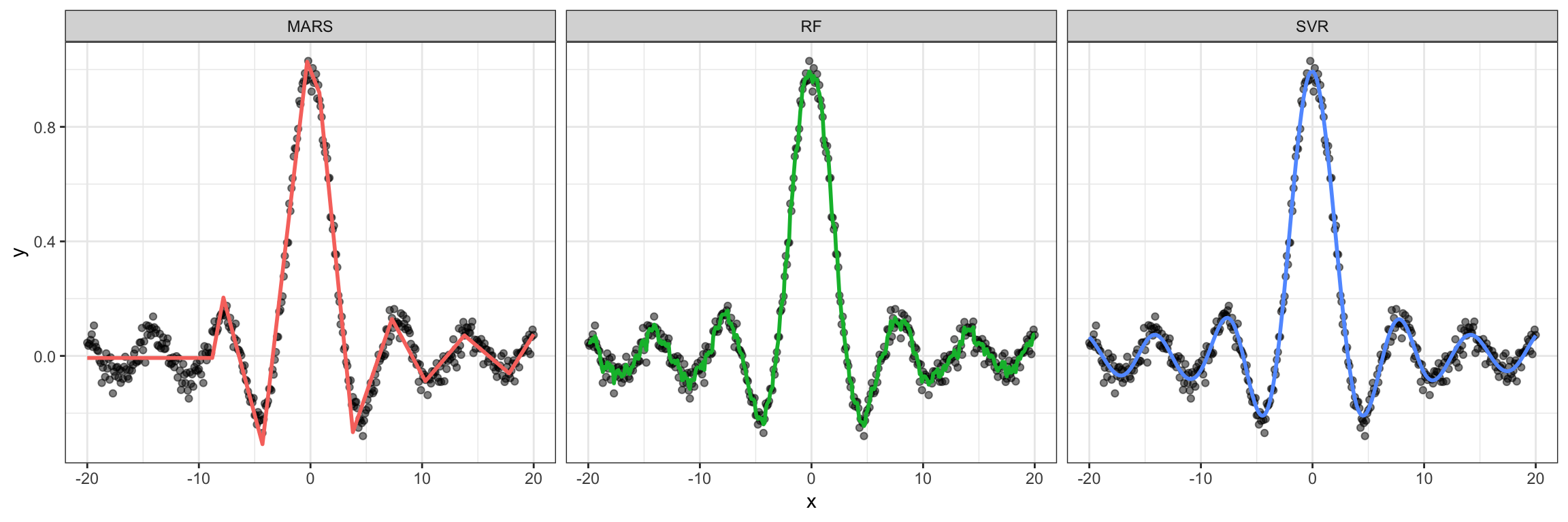
Figure 14.10: Simulated sine

Applying support vector regression to the Ames housing example is left as an exercise for the reader on the book’s website.

14.4 Job attrition example

Returning to the employee attrition example, we tune and fit an SVM with a radial basis kernel (recall our earlier rule of thumb regarding kernel functions). Recall that the radial basis kernel has two hyperparameters: \(\sigma\) and \(C\). While we can use k-fold CV to find good estimates of both parameters, hyperparameter tuning can be time consuming for SVMs⁴¹. Fortunately, it is possible to use the training data to find a good estimate of \(\sigma\). This is provided by the kernlab::sigest() function. This function estimates the range of \(\sigma\) values which would return good results when used with a radial basis SVM. Ideally, any value within the range of estimates returned by this function should produce reasonable results. This is the approach taken by caret’s train() function when method = "svmRadialSigma", which we use below. Also, note that a reasonable search grid for the cost parameter \(C\) is an exponentially growing series, for example \(2^{-2}, 2^{-1}, 2^{0}, 2^{1}, 2^{2},\) etc. See caret::getModelInfo("svmRadialSigma") for details.

Next, we’ll use caret’s train() function to tune and train an SVM using the radial basis kernel function with autotuning for the \(\sigma\) parameter (i.e., "svmRadialSigma") and 10-fold CV.

# Tune an SVM with radial basis kernel
set.seed(1854)  # for reproducibility
churn_svm <- train(
  Attrition ~ ., 
  data = churn_train,
  method = "svmRadial",               
  preProcess = c("center", "scale"),  
  trControl = trainControl(method = "cv", number = 10),
  tuneLength = 10
)

Plotting the results, we see that smaller values of the cost parameter (\(C \approx\) 2–8) provide better cross-validated accuracy scores for these training data:

# Plot results
ggplot(churn_svm) + theme_light()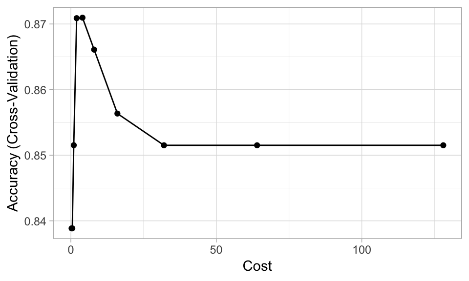

# Print results
churn_svm$results
##          sigma      C  Accuracy     Kappa  AccuracySD   KappaSD
## 1  0.009590249   0.25 0.8388542 0.0000000 0.004089627 0.0000000
## 2  0.009590249   0.50 0.8388542 0.0000000 0.004089627 0.0000000
## 3  0.009590249   1.00 0.8515233 0.1300469 0.014427649 0.1013069
## 4  0.009590249   2.00 0.8708857 0.3526368 0.023749215 0.1449342
## 5  0.009590249   4.00 0.8709611 0.4172884 0.026640331 0.1302496
## 6  0.009590249   8.00 0.8660873 0.4242800 0.026271496 0.1206188
## 7  0.009590249  16.00 0.8563495 0.4012563 0.026866012 0.1298460
## 8  0.009590249  32.00 0.8515138 0.3831775 0.028717623 0.1338717
## 9  0.009590249  64.00 0.8515138 0.3831775 0.028717623 0.1338717
## 10 0.009590249 128.00 0.8515138 0.3831775 0.028717623 0.1338717

14.4.1 Class weights

By default, most classification algorithms treat misclassification costs equally. This is not ideal in situations where one type of misclassification is more important than another or there is a severe class imbalance (which is usually the case). SVMs (as well as most tree-based methods) allow you to assign specific misclassification costs to the different outcomes. In caret and kernlab, this is accomplished via the class.weights argument, which is just a named vector of weights for the different classes. In the employee attrition example, for instance, we might specify

class.weights = c("No" = 1, "Yes" = 10)

in the call to caret::train() or kernlab::ksvm() to make false negatives (i.e., predicting “Yes” when the truth is “No”) ten times more costly than false positives (i.e., predicting “No” when the truth is “Yes”). Cost-sensitive training with SVMs is left as an exercise on the book website.

14.4.2 Class probabilities

SVMs classify new observations by determining which side of the decision boundary they fall on; consequently, they do not automatically provide predicted class probabilities! In order to obtain predicted class probabilities from an SVM, additional parameters need to be estimated as described in Platt (1999). In practice, predicted class probabilities are often more useful than the predicted class labels. For instance, we would need the predicted class probabilities if we were using an optimization metric like AUC (Chapter 2), as opposed to classification accuracy. In that case, we can set prob.model = TRUE in the call to kernlab::ksvm() or classProbs = TRUE in the call to caret::trainControl() (for details, see ?kernlab::ksvm and the references therein):

# Control params for SVM
ctrl <- trainControl(
  method = "cv", 
  number = 10, 
  classProbs = TRUE,                 
  summaryFunction = twoClassSummary  # also needed for AUC/ROC
)

# Tune an SVM
set.seed(5628)  # for reproducibility
churn_svm_auc <- train(
  Attrition ~ ., 
  data = churn_train,
  method = "svmRadial",               
  preProcess = c("center", "scale"),  
  metric = "ROC",  # area under ROC curve (AUC)       
  trControl = ctrl,
  tuneLength = 10
)

# Print results
churn_svm_auc$results
##          sigma      C       ROC      Sens      Spec      ROCSD      SensSD     SpecSD
## 1  0.009727585   0.25 0.8379109 0.9675488 0.3933824 0.06701067 0.012073306 0.11466031
## 2  0.009727585   0.50 0.8376397 0.9652767 0.3761029 0.06694554 0.010902039 0.14775214
## 3  0.009727585   1.00 0.8377081 0.9652633 0.4055147 0.06725101 0.007798768 0.09871169
## 4  0.009727585   2.00 0.8343294 0.9756750 0.3459559 0.06803483 0.012712528 0.14320366
## 5  0.009727585   4.00 0.8200427 0.9745255 0.3452206 0.07188838 0.013092221 0.12082675
## 6  0.009727585   8.00 0.8123546 0.9699278 0.3327206 0.07582032 0.013513393 0.11819788
## 7  0.009727585  16.00 0.7915612 0.9756883 0.2849265 0.07791598 0.010094292 0.10700782
## 8  0.009727585  32.00 0.7846566 0.9745255 0.2845588 0.07752526 0.010615423 0.08923723
## 9  0.009727585  64.00 0.7848594 0.9745255 0.2845588 0.07741087 0.010615423 0.09848550
## 10 0.009727585 128.00 0.7848594 0.9733895 0.2783088 0.07741087 0.010922892 0.10913126

Similar to before, we see that smaller values of the cost parameter \(C\) (\(C \approx 2-4\)) provide better cross-validated AUC scores on the training data. Also, notice how in addition to ROC we also get the corresponding sensitivity (true positive rate) and specificity (true negative rate). In this case, sensitivity (column Sens) refers to the proportion of Nos correctly predicted as No and specificity (column Spec) refers to the proportion of Yess correctly predicted as Yes. We can succinctly describe the different classification metrics using caret’s confusionMatrix() function (see ?caret::confusionMatrix for details):

confusionMatrix(churn_svm_auc)
## Cross-Validated (10 fold) Confusion Matrix 
## 
## (entries are percentual average cell counts across resamples)
##  
##           Reference
## Prediction   No  Yes
##        No  81.2  9.8
##        Yes  2.7  6.3
##                             
##  Accuracy (average) : 0.8748

In this case it is clear that we do a far better job at predicting the Nos.

14.5 Feature interpretation

Like many other ML algorithms, SVMs do not emit any natural measures of feature importance; however, we can use the vip package to quantify the importance of each feature using the permutation approach described later on in Chapter 16 (the iml and DALEX packages could also be used).

Our metric function should reflect the fact that we trained the model using AUC. Any custom metric function provided to vip() should have the arguments actual and predicted (in that order). We illustrate this below where we wrap the auc() function from the ModelMetrics package (Hunt 2018):

Since we are using AUC as our metric, our prediction wrapper function should return the predicted class probabilities for the reference class of interest. In this case, we’ll use "Yes" as the reference class (to do this we’ll specify reference_class = "Yes" in the call to vip::vip()). Our prediction function looks like:

prob_yes <- function(object, newdata) {
  predict(object, newdata = newdata, type = "prob")[, "Yes"]
}

To compute the variable importance scores we just call vip() with method = "permute" and pass our previously defined predictions wrapper to the pred_wrapper argument:

# Variable importance plot
set.seed(2827)  # for reproducibility
vip(churn_svm_auc, method = "permute", nsim = 5, train = churn_train, 
    target = "Attrition", metric = "auc", reference_class = "Yes", 
    pred_wrapper = prob_yes)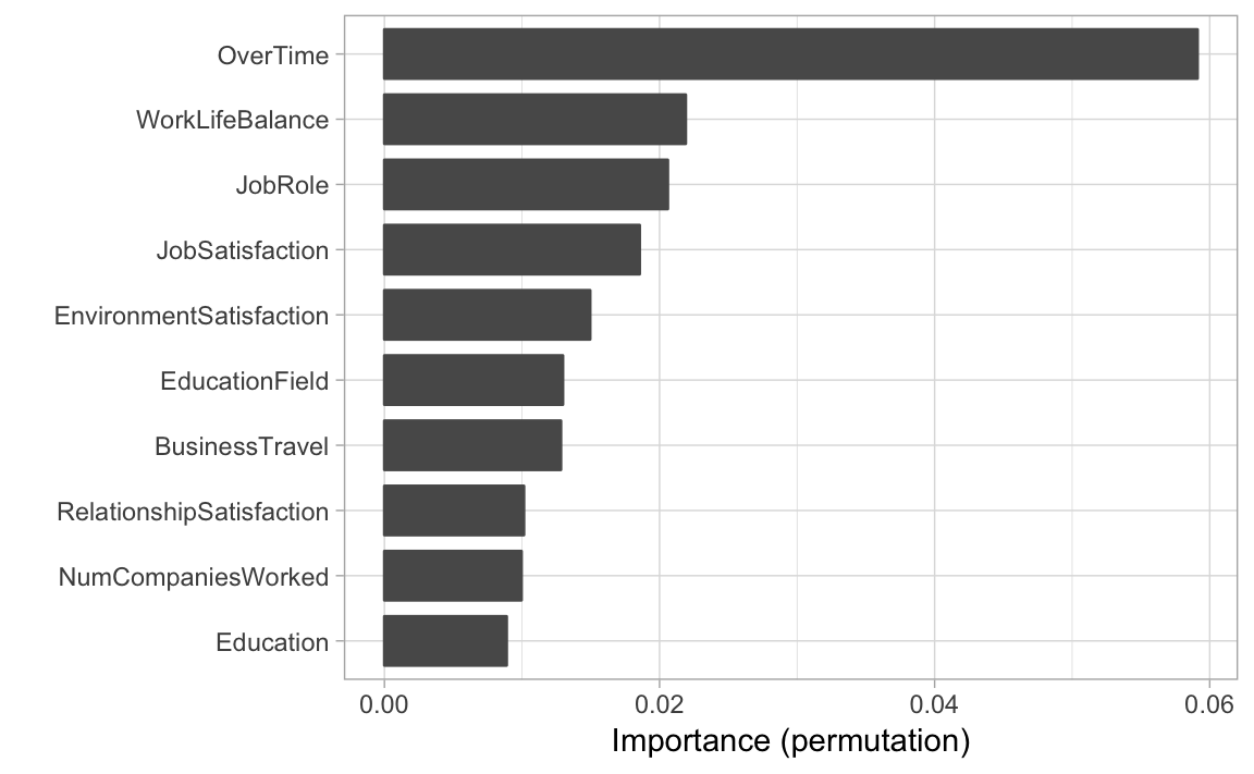

The results indicate that OverTime (Yes/No) is the most important feature in predicting attrition. Next, we use the pdp package to construct PDPs for the top four features according to the permutation-based variable importance scores (notice we set prob = TRUE in the call to pdp::partial() so that the feature effect plots are on the probability scale; see ?pdp::partial for details). Additionally, since the predicted probabilities from our model come in two columns (No and Yes), we specify which.class = 2 so that our interpretation is in reference to predicting Yes:

features <- c("OverTime", "WorkLifeBalance", 
              "JobSatisfaction", "JobRole")
pdps <- lapply(features, function(x) {
  partial(churn_svm_auc, pred.var = x, which.class = 2,  
          prob = TRUE, plot = TRUE, plot.engine = "ggplot2") +
    coord_flip()
})
grid.arrange(grobs = pdps,  ncol = 2)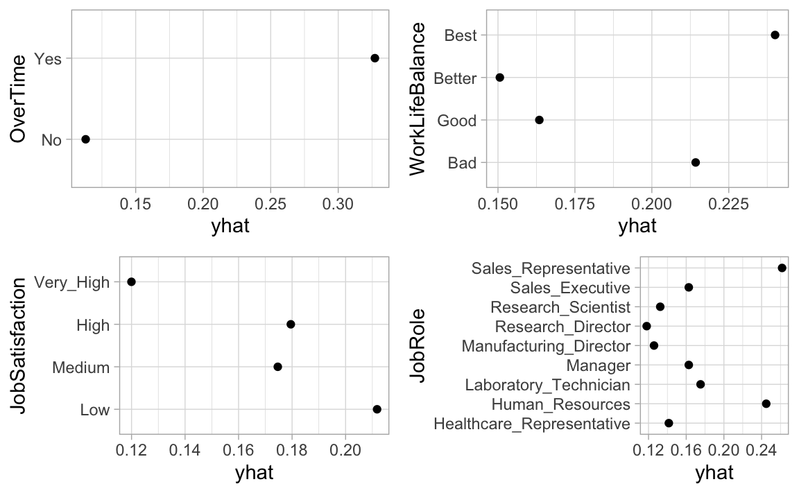

For instance, we see that employees with a low job satisfaction level have the highest probability of attriting, while those with a very high level of satisfaction tend to have the lowest probability.

14.6 Final thoughts

SVMs have a number of advantages compared to other ML algorithms described in this book. First off, they attempt to directly maximize generalizability (i.e., accuracy). Since SVMs are essentially just convex optimization problems, we’re always guaranteed to find a global optimum (as opposed to potentially getting stuck in local optima as with DNNs). By softening the margin using a budget (or cost) parameter (\(C\)), SVMs are relatively robust to outliers. And finally, using kernel functions, SVMs are flexible enough to adapt to complex nonlinear decision boundaries (i.e., they can flexibly model nonlinear relationships). However, SVMs do carry a few disadvantages as well. For starters, they can be slow to train on tall data (i.e., \(n >> p\)). This is because SVMs essentially have to estimate at least one parameter for each row in the training data! Secondly, SVMs only produce predicted class labels; obtaining predicted class probabilities requires additional adjustments and computations not covered in this chapter. Lastly, special procedures (e.g., OVA and OVO) have to be used to handle multinomial classification problems with SVMs.

References

Hastie, Trevor. 2016. Svmpath: The Svm Path Algorithm. https://CRAN.R-project.org/package=svmpath.

Hunt, Tyler. 2018. ModelMetrics: Rapid Calculation of Model Metrics. https://CRAN.R-project.org/package=ModelMetrics.

Karatzoglou, Alexandros, Alex Smola, Kurt Hornik, and Achim Zeileis. 2004. “Kernlab – an S4 Package for Kernel Methods in R.” Journal of Statistical Software 11 (9): 1–20. http://www.jstatsoft.org/v11/i09/.

Meyer, David, Evgenia Dimitriadou, Kurt Hornik, Andreas Weingessel, and Friedrich Leisch. 2019. E1071: Misc Functions of the Department of Statistics, Probability Theory Group (Formerly: E1071), Tu Wien. https://CRAN.R-project.org/package=e1071.

Platt, John C. 1999. “Probabilistic Outputs for Support Vector Machines and Comparisons to Regularized Likelihood Methods.” In Advances in Large Margin Classifiers, 61–74. MIT Press.

---

40. The convex hull of a set of points in 2-D space can be thought of as the shape formed by a rubber band stretched around the data. This of course can be generalized to higher dimensions (e.g., a rubber membrane stretched around a cloud of points in 3-D space).↩

41. SVMs typically have to estimate at least as many parameters as there are rows in the training data. Hence, SVMs are more commonly used in wide data situations.↩