Chapter 17 Principal Components Analysis
Principal components analysis (PCA) is a method for finding low-dimensional representations of a data set that retain as much of the original variation as possible. The idea is that each of the n observations lives in p-dimensional space, but not all of these dimensions are equally interesting. In PCA we look for a smaller number of dimensions that are as interesting as possible, where the concept of interesting is measured by the amount that the observations vary along each dimension. Each of the new dimensions found in PCA is a linear combination of the original p features. The hope is to use a small subset of these linear feature combinations in further analysis while retaining most of the information present in the original data.
17.1 Prerequisites
This chapter leverages the following packages.
library(dplyr)       # basic data manipulation and plotting
library(ggplot2)     # data visualization
library(h2o)         # performing dimension reduction
To illustrate dimension reduction techniques, we’ll use the my_basket data set (Section 1.4). This data set identifies items and quantities purchased for 2,000 transactions from a grocery store. The objective is to identify common groupings of items purchased together.
url <- "https://koalaverse.github.io/homlr/data/my_basket.csv"
my_basket <- readr::read_csv(url)
dim(my_basket)
## [1] 2000   42
To perform dimension reduction techniques in R, generally, the data should be prepared as follows:
- Data are in tidy format per Wickham and others (2014);
- Any missing values in the data must be removed or imputed;
- Typically, the data must all be numeric values (e.g., one-hot, label, ordinal encoding categorical features);
- Numeric data should be standardized (e.g., centered and scaled) to make features comparable.
The my_basket data already fullfills these requirements. However, some of the packages we’ll use to perform dimension reduction tasks have built-in capabilities to impute missing data, numerically encode categorical features (typically one-hot encode), and standardize the features.
17.2 The idea
Dimension reduction methods, such as PCA, focus on reducing the feature space, allowing most of the information or variability in the data set to be explained using fewer features; in the case of PCA, these new features will also be uncorrelated. For example, among the 42 variables within the my_basket data set, 23 combinations of variables have moderate correlation (\(\geq 0.25\)) with each other. Looking at the table below, we see that some of these combinations may be represented with smaller dimension categories (e.g., soda, candy, breakfast, and italian food)
| Item 1 | Item 2 | Correlation |
|---|---|---|
| cheese | mayonnaise | 0.345 |
| bulmers | fosters | 0.335 |
| cheese | bread | 0.320 |
| lasagna | pizza | 0.316 |
| pepsi | coke | 0.309 |
| red.wine | fosters | 0.308 |
| milk | muesli | 0.302 |
| mars | twix | 0.301 |
| red.wine | bulmers | 0.298 |
| bulmers | kronenbourg | 0.289 |
| milk | tea | 0.288 |
| red.wine | kronenbourg | 0.286 |
| 7up | coke | 0.282 |
| spinach | broccoli | 0.282 |
| mayonnaise | bread | 0.278 |
| peas | potatoes | 0.271 |
| peas | carrots | 0.270 |
| tea | instant.coffee | 0.270 |
| milk | instant.coffee | 0.267 |
| bread | lettuce | 0.264 |
| twix | kitkat | 0.259 |
| mars | kitkat | 0.255 |
| muesli | instant.coffee | 0.251 |
We often want to explain common attributes such as these in a lower dimensionality than the original data. For example, when we purchase soda we may often buy multiple types at the same time (e.g., Coke, Pepsi, and 7UP). We could reduce these variables to one latent variable (i.e., unobserved feature) called “soda”. This can help in describing many features in our data set and it can also remove multicollinearity, which can often improve predictive accuracy in downstream supervised models.
So how do we identify variables that could be grouped into a lower dimension? One option includes examining pairwise scatterplots of each variable against every other variable and identifying co-variation. Unfortunately, this is tedious and becomes excessive quickly even with a small number of variables (given \(p\) variables there are \(p(p-1)/2\) possible scatterplot combinations). For example, since the my_basket data has 42 numeric variables, we would need to examine \(42(42-1)/2 = 861\) scatterplots! Fortunately, better approaches exist to help represent our data using a smaller dimension.
The PCA method was first published in 1901 (Pearson 1901) and has been a staple procedure for dimension reduction for decades. PCA examines the covariance among features and combines multiple features into a smaller set of uncorrelated variables. These new features, which are weighted combinations of the original predictor set, are called principal components (PCs) and hopefully a small subset of them explain most of the variability of the full feature set. The weights used to form the PCs reveal the relative contributions of the original features to the new PCs.
17.3 Finding principal components
The first principal component of a set of features \(X_1\), \(X_2\), …, \(X_p\) is the linear combination of the features
\[\begin{equation} \tag{17.1} Z_{1} = \phi_{11}X_{1} + \phi_{21}X_{2} + ... + \phi_{p1}X_{p}, \end{equation}\]
that has the largest variance. Here \(\phi_1 = \left(\phi_{11}, \phi_{21}, \dots, \phi_{p1}\right)\) is the loading vector for the first principal component. The \(\phi\) are normalized so that \(\sum_{j=1}^{p}{\phi_{j1}^{2}} = 1\). After the first principal component \(Z_1\) has been determined, we can find the second principal component \(Z_2\). The second principal component is the linear combination of \(X_1, \dots , X_p\) that has maximal variance out of all linear combinations that are uncorrelated with \(Z_1\):
\[\begin{equation} \tag{17.2} Z_{2} = \phi_{12}X_{1} + \phi_{22}X_{2} + ... + \phi_{p2}X_{p} \end{equation}\]
where again we define \(\phi_2 = \left(\phi_{12}, \phi_{22}, \dots, \phi_{p2}\right)\) as the loading vector for the second principal component. This process proceeds until all p principal components are computed. So how do we calculate \(\phi_1, \phi_2, \dots, \phi_p\) in practice?. It can be shown, using techniques from linear algebra45, that the eigenvector corresponding to the largest eigenvalue of the feature covariance matrix is the set of loadings that explains the greatest proportion of feature variability.46
An illustration provides a more intuitive grasp on principal components. Assume we have two features that have moderate (0.56, say) correlation. We can explain the covariation of these variables in two dimensions (i.e., using PC 1 and PC 2). We see that the greatest covariation falls along the first PC, which is simply the line that minimizes the total squared distance from each point to its orthogonal projection onto the line. Consequently, we can explain the vast majority (93% to be exact) of the variability between feature 1 and feature 2 using just the first PC.
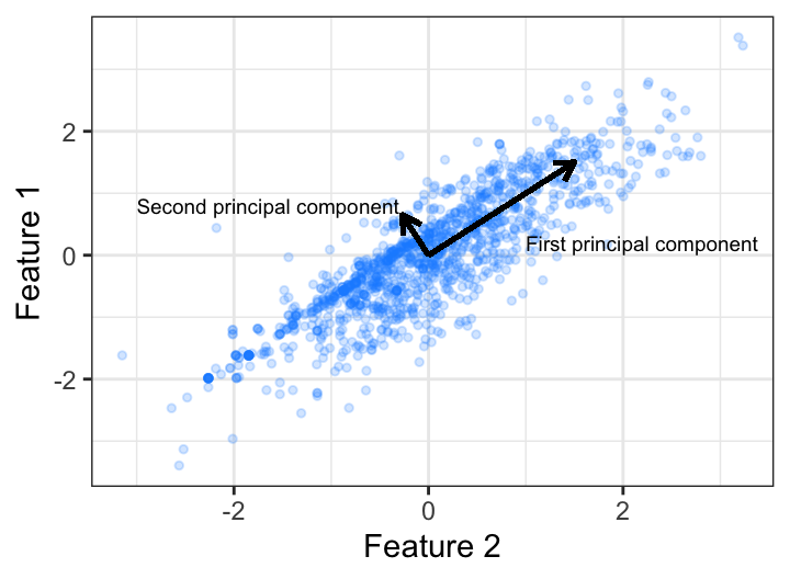
Figure 17.1: Principal components of two features that have 0.56 correlation.
We can extend this to three variables, assessing the relationship among features 1, 2, and 3. The first two PC directions span the plane that best fits the variability in the data. It minimizes the sum of squared distances from each point to the plan. As more dimensions are added, these visuals are not as intuitive but we’ll see shortly how we can still use PCA to extract and visualize important information.
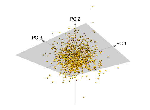
Figure 17.2: Principal components of three features.
17.4 Performing PCA in R
There are several built-in and external packages to perform PCA in R. We recommend to use h2o as it provides consistency across the dimension reduction methods we’ll discuss later and it also automates much of the data preparation steps previously discussed (i.e., standardizing numeric features, imputing missing values, and encoding categorical features).
Let’s go ahead and start up h2o:
h2o.no_progress()  # turn off progress bars for brevity
h2o.init(max_mem_size = "5g")  # connect to H2O instance
First, we convert our my_basket data frame to an appropriate h2o object and then use h2o.prcomp() to perform PCA. A few of the important arguments you can specify in h2o.prcomp() include:
pca_method: Character string specifying which PC method to use. there are actually a few different approaches to calculating principal components (PCs). When your data contains mostly numeric data (such asmy_basket), its best to usepca_method = "GramSVD". When your data contain many categorical variables (or just a few categorical variables with high cardinality) we recommend you usepca_method = "GLRM".k: Integer specifying how many PCs to compute. It’s best to create the same number of PCs as there are features and we will see shortly how to identify the number of PCs to use, where the number of PCs is less than the number of features.transform: Character string specifying how (if at all) your data should be standardized.impute_missing: Logical specifying whether or not to impute missing values; if your data have missing values, this will impute them with the corresponding column mean.max_runtime_secs: Number specifying the max run time (in seconds); when working with large data sets this will limit the runtime for model training.
When your data contains mostly numeric data (such as my_basket), its best to use pca_method = “GramSVD”. When your data contain many categorical variables (or just a few categorical variables with high cardinality) we recommend to use pca_method = “GLRM”.
# convert data to h2o object
my_basket.h2o <- as.h2o(my_basket)

# run PCA
my_pca <- h2o.prcomp(
  training_frame = my_basket.h2o,
  pca_method = "GramSVD",
  k = ncol(my_basket.h2o),
  transform = "STANDARDIZE",
  impute_missing = TRUE,
  max_runtime_secs = 1000
)
Our model object (my_pca) contains several pieces of information that we can extract (you can view all information with glimpse(my_pca)). The most important information is stored in my_pca@model$importance (which is the same output that gets printed when looking at our object’s printed output). This information includes each PC, the standard deviation of each PC, as well as the proportion and cumulative proportion of variance explained with each PC.
my_pca
## Model Details:
## ==============
##
## H2ODimReductionModel: pca
## Model ID:  PCA_model_R_1536152543598_1
## Importance of components:
##                             pc1      pc2      pc3      pc4      pc5      pc6      pc7      pc8      pc9
## Standard deviation     1.513919 1.473768 1.459114 1.440635 1.435279 1.411544 1.253307 1.026387 1.010238
## Proportion of Variance 0.054570 0.051714 0.050691 0.049415 0.049048 0.047439 0.037400 0.025083 0.024300
## Cumulative Proportion  0.054570 0.106284 0.156975 0.206390 0.255438 0.302878 0.340277 0.365360 0.389659
##                            pc10     pc11     pc12     pc13     pc14     pc15     pc16     pc17     pc18
## Standard deviation     1.007253 0.988724 0.985320 0.970453 0.964303 0.951610 0.947978 0.944826 0.932943
## Proportion of Variance 0.024156 0.023276 0.023116 0.022423 0.022140 0.021561 0.021397 0.021255 0.020723
## Cumulative Proportion  0.413816 0.437091 0.460207 0.482630 0.504770 0.526331 0.547728 0.568982 0.589706
##                            pc19     pc20     pc21     pc22     pc23     pc24     pc25     pc26     pc27
## Standard deviation     0.931745 0.924207 0.917106 0.908494 0.903247 0.898109 0.894277 0.876167 0.871809
## Proportion of Variance 0.020670 0.020337 0.020026 0.019651 0.019425 0.019205 0.019041 0.018278 0.018096
## Cumulative Proportion  0.610376 0.630713 0.650739 0.670390 0.689815 0.709020 0.728061 0.746339 0.764436
##                            pc28     pc29     pc30     pc31     pc32     pc33     pc34     pc35     pc36
## Standard deviation     0.865912 0.855036 0.845130 0.842818 0.837655 0.826422 0.818532 0.813796 0.804380
## Proportion of Variance 0.017852 0.017407 0.017006 0.016913 0.016706 0.016261 0.015952 0.015768 0.015405
## Cumulative Proportion  0.782288 0.799695 0.816701 0.833614 0.850320 0.866581 0.882534 0.898302 0.913707
##                            pc37     pc38     pc39     pc40     pc41     pc42
## Standard deviation     0.796073 0.793781 0.780615 0.778612 0.763433 0.749696
## Proportion of Variance 0.015089 0.015002 0.014509 0.014434 0.013877 0.013382
## Cumulative Proportion  0.928796 0.943798 0.958307 0.972741 0.986618 1.000000
##
##
## H2ODimReductionMetrics: pca
##
## No model metrics available for PCA
Naturally, the first PC (PC1) captures the most variance followed by PC2, then PC3, etc. We can identify which of our original features contribute to the PCs by assessing the loadings. The loadings for the first PC represent \(\phi_{11}, \phi_{21}, \dots, \phi_{p1}\) in Equation (17.1). Thus, these loadings represent each features influence on the associated PC. If we plot the loadings for PC1 we see that the largest contributing features are mostly adult beverages (and apparently eating candy bars, smoking, and playing the lottery are also associated with drinking!).
my_pca@model$eigenvectors %>%
  as.data.frame() %>%
  mutate(feature = row.names(.)) %>%
  ggplot(aes(pc1, reorder(feature, pc1))) +
  geom_point()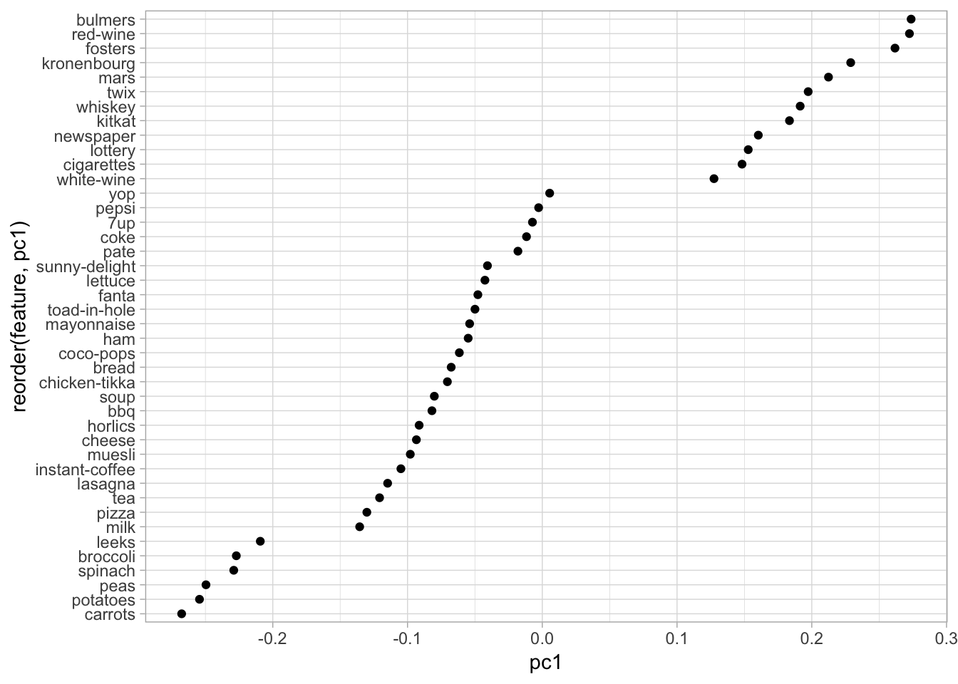
Figure 17.3: Feature loadings illustrating the influence that each variable has on the first principal component.
We can also compare PCs against one another. For example, Figure 17.4 shows how the different features contribute to PC1 and PC2. We can see distinct groupings of features and how they contribute to both PCs. For example, adult beverages (e.g., whiskey and wine) have a positive contribution to PC1 but have a smaller and negative contribution to PC2. This means that transactions that include purchases of adult beverages tend to have larger than average values for PC1 but smaller than average for PC2.
my_pca@model$eigenvectors %>%
  as.data.frame() %>%
  mutate(feature = row.names(.)) %>%
  ggplot(aes(pc1, pc2, label = feature)) +
  geom_text()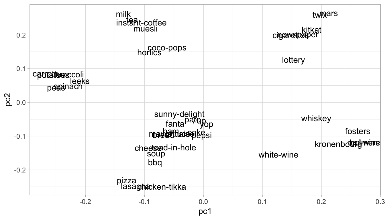
Figure 17.4: Feature contribution for principal components one and two.
17.5 Selecting the number of principal components
So far we have computed PCs and gained a little understanding of what the results initially tell us. However, a primary goal in PCA is dimension reduction (in this case, feature reduction). In essence, we want to come out of PCA with fewer components than original features, and with the caveat that these components explain us as much variation as possible about our data. But how do we decide how many PCs to keep? Do we keep the first 10, 20, or 40 PCs?
There are three common approaches in helping to make this decision:
- Eigenvalue criterion
- Proportion of variance explained criterion
- Scree plot criterion
17.5.1 Eigenvalue criterion
The sum of the eigenvalues is equal to the number of variables entered into the PCA; however, the eigenvalues will range from greater than one to near zero. An eigenvalue of 1 means that the principal component would explain about one variable’s worth of the variability. The rationale for using the eigenvalue criterion is that each component should explain at least one variable’s worth of the variability, and therefore, the eigenvalue criterion states that only components with eigenvalues greater than 1 should be retained.
h2o.prcomp() automatically computes the standard deviations of the PCs, which is equal to the square root of the eigenvalues. Therefore, we can compute the eigenvalues easily and identify PCs where the sum of eigenvalues is greater than or equal to 1. Consequently, using this criteria would have us retain the first 10 PCs in my_basket (see Figure 17.5).
# Compute eigenvalues
eigen <- my_pca@model$importance["Standard deviation", ] %>%
  as.vector() %>%
  .^2

# Sum of all eigenvalues equals number of variables
sum(eigen)
## [1] 42

# Find PCs where the sum of eigenvalues is greater than or equal to 1
which(eigen >= 1)
##  [1]  1  2  3  4  5  6  7  8  9 10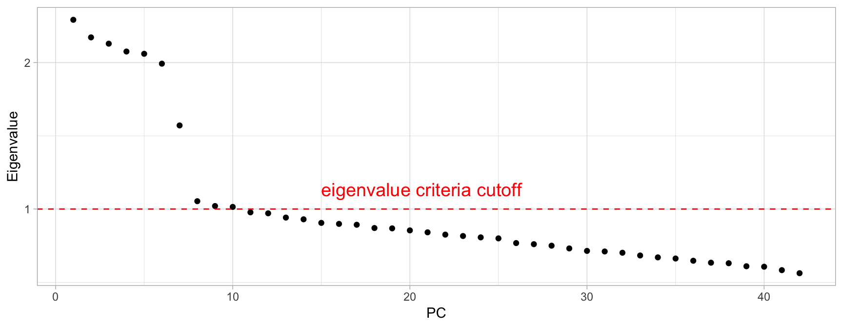
Figure 17.5: Eigenvalue criterion keeps all principal components where the sum of the eigenvalues are above or equal to a value of one.
17.5.2 Proportion of variance explained criterion
The proportion of variance explained (PVE) identifies the optimal number of PCs to keep based on the total variability that we would like to account for. Mathematically, the PVE for the m-th PC is calculated as:
\[\begin{equation} \tag{17.3} PVE = \frac{\sum_{i=1}^{n}(\sum_{j=1}^{p}{\phi_{jm}x_{ij}})^{2}}{\sum_{j=1}^{p}\sum_{i=1}^{n}{x_{ij}^{2}}} \end{equation}\]
h2o.prcomp() provides us with the PVE and also the cumulative variance explained (CVE), so we just need to extract this information and plot it (see Figure 17.6).
# Extract and plot PVE and CVE
data.frame(
  PC  = my_pca@model$importance %>% seq_along(),
  PVE = my_pca@model$importance %>% .[2,] %>% unlist(),
  CVE = my_pca@model$importance %>% .[3,] %>% unlist()
) %>%
  tidyr::gather(metric, variance_explained, -PC) %>%
  ggplot(aes(PC, variance_explained)) +
  geom_point() +
  facet_wrap(~ metric, ncol = 1, scales = "free")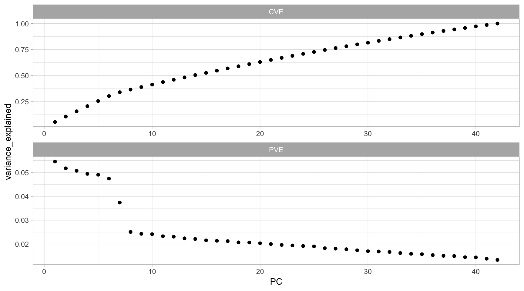
Figure 17.6: PVE criterion keeps all principal components that are above or equal to a pre-specified threshold of total variability explained.
The first PCt in our example explains 5.46% of the feature variability, and the second principal component explains 5.17%. Together, the first two PCs explain 10.63% of the variability. Thus, if an analyst desires to choose the number of PCs required to explain at least 75% of the variability in our original data then they would choose the first 27 components.
# How many PCs required to explain at least 75% of total variability
min(which(ve$CVE >= 0.75))
## [1] 27
What amount of variability is reasonable? This varies by application and the data being used. However, when the PCs are being used for descriptive purposes only, such as customer profiling, then the proportion of variability explained may be lower than otherwise. When the PCs are to be used as derived features for models downstream, then the PVE should be as much as can conveniently be achieved, given any constraints.
17.5.3 Scree plot criterion
A scree plot shows the eigenvalues or PVE for each individual PC. Most scree plots look broadly similar in shape, starting high on the left, falling rather quickly, and then flattening out at some point. This is because the first component usually explains much of the variability, the next few components explain a moderate amount, and the latter components only explain a small fraction of the overall variability. The scree plot criterion looks for the “elbow” in the curve and selects all components just before the line flattens out, which looks like eight in our example (see Figure 17.7).
data.frame(
  PC  = my_pca@model$importance %>% seq_along,
  PVE = my_pca@model$importance %>% .[2,] %>% unlist()
) %>%
  ggplot(aes(PC, PVE, group = 1, label = PC)) +
  geom_point() +
  geom_line() +
  geom_text(nudge_y = -.002)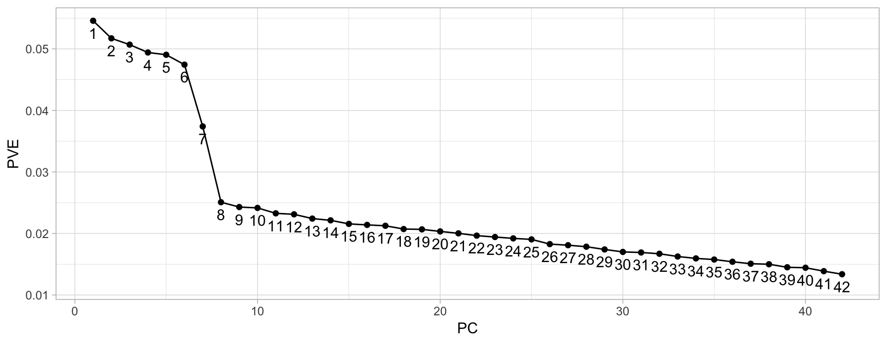
Figure 17.7: Scree plot criterion looks for the ‘elbow’ in the curve and keeps all principal components before the line flattens out.
17.6 Final thoughts
So how many PCs should we use in the my_basket example? The frank answer is that there is no one best method for determining how many components to use. In this case, differing criteria suggest to retain 8 (scree plot criterion), 10 (eigenvalue criterion), and 26 (based on a 75% of variance explained requirement) components. The number you go with depends on your end objective and analytic workflow. If we were merely trying to profile customers we would probably use 8 or 10, if we were performing dimension reduction to feed into a downstream predictive model we would likely retain 26 or more (the exact number being based on, for example, the CV results in the supervised modeling process). This is part of the challenge with unsupervised modeling, there is more subjectivity in modeling results and interpretation.
Traditional PCA has a few disadvantages worth keeping in mind. First, PCA can be highly affected by outliers. There have been many robust variants of PCA that act to iteratively discard data points that are poorly described by the initial components (see, for example, Luu, Blum, and Privé (2019) and Erichson, Zheng, and Aravkin (2018)). In Chapter 18 we discuss an alternative dimension reduction procedure that takes outliers into consideration, and in Chapter 19 we illustrate a procedure to help identify outliers.
Also, note in Figures 17.1 and 17.2 that our PC directions are linear. Consequently, traditional PCA does not perform as well in very high dimensional space where complex nonlinear patterns often exist. Kernel PCA implements the kernel trick discussed in Chapter 14 and makes it possible to perform complex nonlinear projections of dimensionality reduction. See Karatzoglou, Smola, and Hornik (2018) for an implementation of kernel PCA in R. Chapters 18 and 19 discuss two methods that allow us to reduce the feature space while also capturing nonlinearity.
References
Erichson, N. Benjamin, Peng Zheng, and Sasha Aravkin. 2018. Sparsepca: Sparse Principal Component Analysis (Spca). https://CRAN.R-project.org/package=sparsepca.
Karatzoglou, Alexandros, Alex Smola, and Kurt Hornik. 2018. Kernlab: Kernel-Based Machine Learning Lab. https://CRAN.R-project.org/package=kernlab.
Luu, Keurcien, Michael Blum, and Florian Privé. 2019. Pcadapt: Fast Principal Component Analysis for Outlier Detection. https://CRAN.R-project.org/package=pcadapt.
Pearson, Karl. 1901. “LIII. On Lines and Planes of Closest Fit to Systems of Points in Space.” The London, Edinburgh, and Dublin Philosophical Magazine and Journal of Science 2 (11). Taylor & Francis: 559–72.
Wickham, Hadley, and others. 2014. “Tidy Data.” Journal of Statistical Software 59 (10). Foundation for Open Access Statistics: 1–23.
Linear algebra is fundamental to mastering many advanced concepts in statistics and machine learning, but is out of the scope of this book.↩
In particular, the PCs can be found using an eigen decomposition applied to the special matrix \(\boldsymbol{X}'\boldsymbol{X}\) (where \(\boldsymbol{X}\) is an \(n \times p\) matrix consisting of the centered feature values).↩