Chapter 21 Hierarchical Clustering
Hierarchical clustering is an alternative approach to k-means clustering for identifying groups in a data set. In contrast to k-means, hierarchical clustering will create a hierarchy of clusters and therefore does not require us to pre-specify the number of clusters. Furthermore, hierarchical clustering has an added advantage over k-means clustering in that its results can be easily visualized using an attractive tree-based representation called a dendrogram.
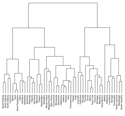
Figure 21.1: Illustrative dendrogram.
21.1 Prerequisites
For this chapter we’ll use the following packages:
# Helper packages
library(dplyr)       # for data manipulation
library(ggplot2)     # for data visualization

# Modeling packages
library(cluster)     # for general clustering algorithms
library(factoextra)  # for visualizing cluster results
The major concepts of hierarchical clustering will be illustrated using the Ames housing data. For simplicity we’ll just use the 34 numeric features but refer to our discussion in Section 20.7 if you’d like to replicate this analysis with the full set of features. Since these features are measured on significantly different magnitudes we standardize the data first:
ames_scale <- AmesHousing::make_ames() %>%
  select_if(is.numeric) %>%  # select numeric columns
  select(-Sale_Price) %>%    # remove target column
  mutate_all(as.double) %>%  # coerce to double type
  scale()                    # center & scale the resulting columns
21.2 Hierarchical clustering algorithms
Hierarchical clustering can be divided into two main types:
- Agglomerative clustering: Commonly referred to as AGNES (AGglomerative NESting) works in a bottom-up manner. That is, each observation is initially considered as a single-element cluster (leaf). At each step of the algorithm, the two clusters that are the most similar are combined into a new bigger cluster (nodes). This procedure is iterated until all points are a member of just one single big cluster (root) (see Figure 21.2). The result is a tree which can be displayed using a dendrogram.
- Divisive hierarchical clustering: Commonly referred to as DIANA (DIvise ANAlysis) works in a top-down manner. DIANA is like the reverse of AGNES. It begins with the root, in which all observations are included in a single cluster. At each step of the algorithm, the current cluster is split into two clusters that are considered most heterogeneous. The process is iterated until all observations are in their own cluster.
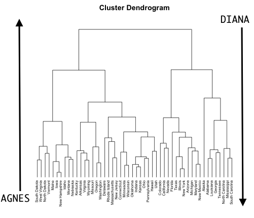
Figure 21.2: AGNES (bottom-up) versus DIANA (top-down) clustering.
Similar to k-means (Chapter 20), we measure the (dis)similarity of observations using distance measures (e.g., Euclidean distance, Manhattan distance, etc.); the Euclidean distance is most commonly the default. However, a fundamental question in hierarchical clustering is: How do we measure the dissimilarity between two clusters of observations? A number of different cluster agglomeration methods (i.e., linkage methods) have been developed to answer this question. The most common methods are:
- Maximum or complete linkage clustering: Computes all pairwise dissimilarities between the elements in cluster 1 and the elements in cluster 2, and considers the largest value of these dissimilarities as the distance between the two clusters. It tends to produce more compact clusters.
- Minimum or single linkage clustering: Computes all pairwise dissimilarities between the elements in cluster 1 and the elements in cluster 2, and considers the smallest of these dissimilarities as a linkage criterion. It tends to produce long, “loose” clusters.
- Mean or average linkage clustering: Computes all pairwise dissimilarities between the elements in cluster 1 and the elements in cluster 2, and considers the average of these dissimilarities as the distance between the two clusters. Can vary in the compactness of the clusters it creates.
- Centroid linkage clustering: Computes the dissimilarity between the centroid for cluster 1 (a mean vector of length \(p\), one element for each variable) and the centroid for cluster 2.
- Ward’s minimum variance method: Minimizes the total within-cluster variance. At each step the pair of clusters with the smallest between-cluster distance are merged. Tends to produce more compact clusters.
Other methods have been introduced such as measuring cluster descriptors after merging two clusters (Ma et al. 2007; Zhao and Tang 2009; Zhang, Zhao, and Wang 2013) but the above methods are, by far, the most popular and commonly used (Hair 2006).
We can see the differences these approaches produce in the dendrograms displayed in Figure 21.3.
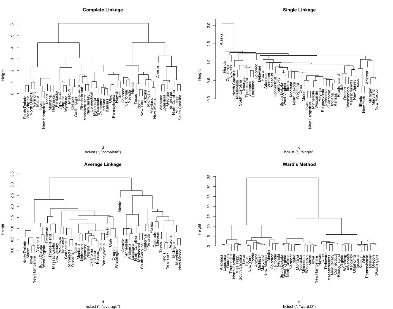
Figure 21.3: Differing hierarchical clustering outputs based on similarity measures.
21.3 Hierarchical clustering in R
There are many functions available in R for hierarchical clustering. The most commonly used functions are stats::hclust() and cluster::agnes() for agglomerative hierarchical clustering (HC) and cluster::diana() for divisive HC.
21.3.1 Agglomerative hierarchical clustering
To perform agglomerative HC with hclust(), we first compute the dissimilarity values with dist() and then feed these values into hclust() and specify the agglomeration method to be used (i.e. "complete", "average", "single", or "ward.D").
# For reproducibility
set.seed(123)

# Dissimilarity matrix
d <- dist(ames_scale, method = "euclidean")

# Hierarchical clustering using Complete Linkage
hc1 <- hclust(d, method = "complete" )plot(hc1, cex = 0.6, hang = -1); however, due to the large number of observations the output is not discernable.
Alternatively, we can use the agnes() function. This function behaves similar to hclust(); however, with the agnes() function you can also get the agglomerative coefficient (AC), which measures the amount of clustering structure found.
Generally speaking, the AC describes the strength of the clustering structure. Values closer to 1 suggest a more balanced clustering structure such as the complete linkage and Ward’s method dendrograms in Figure 21.3. Values closer to 0 suggest less well-formed clusters such as the single linkage dendrogram in Figure 21.3. However, the AC tends to become larger as \(n\) increases, so it should not be used to compare across data sets of very different sizes.
# For reproducibility
set.seed(123)

# Compute maximum or complete linkage clustering with agnes
hc2 <- agnes(ames_scale, method = "complete")

# Agglomerative coefficient
hc2$ac
## [1] 0.926775
This allows us to find certain hierarchical clustering methods that can identify stronger clustering structures. Here we see that Ward’s method identifies the strongest clustering structure of the four methods assessed.
This grid search took a little over 3 minutes.
# methods to assess
m <- c( "average", "single", "complete", "ward")
names(m) <- c( "average", "single", "complete", "ward")

# function to compute coefficient
ac <- function(x) {
  agnes(ames_scale, method = x)$ac
}

# get agglomerative coefficient for each linkage method
purrr::map_dbl(m, ac)
##   average    single  complete      ward
## 0.9139303 0.8712890 0.9267750 0.9766577
21.3.2 Divisive hierarchical clustering
The R function diana() in package cluster allows us to perform divisive hierarchical clustering. diana() works similar to agnes(); however, there is no agglomeration method to provide (see Kaufman and Rousseeuw (2009) for details). As before, a divisive coefficient (DC) closer to one suggests stronger group distinctions. Consequently, it appears that an agglomerative approach with Ward’s linkage provides the optimal results.
# compute divisive hierarchical clustering
hc4 <- diana(ames_scale)

# Divise coefficient; amount of clustering structure found
hc4$dc
## [1] 0.9191094
21.4 Determining optimal clusters
Although hierarchical clustering provides a fully connected dendrogram representing the cluster relationships, you may still need to choose the preferred number of clusters to extract. Fortunately we can execute approaches similar to those discussed for k-means clustering (Section 20.6). The following compares results provided by the elbow, silhouette, and gap statistic methods. There is no definitively clear optimal number of clusters in this case; although, the silhouette method and the gap statistic suggest 8–9 clusters:
# Plot cluster results
p1 <- fviz_nbclust(ames_scale, FUN = hcut, method = "wss",
                   k.max = 10) +
  ggtitle("(A) Elbow method")
p2 <- fviz_nbclust(ames_scale, FUN = hcut, method = "silhouette",
                   k.max = 10) +
  ggtitle("(B) Silhouette method")
p3 <- fviz_nbclust(ames_scale, FUN = hcut, method = "gap_stat",
                   k.max = 10) +
  ggtitle("(C) Gap statistic")

# Display plots side by side
gridExtra::grid.arrange(p1, p2, p3, nrow = 1)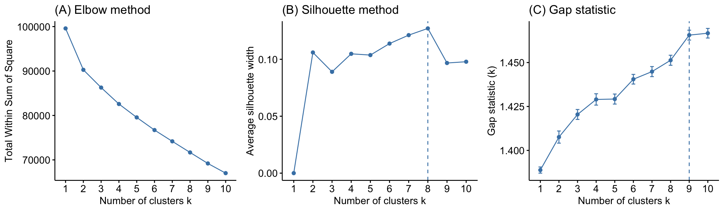
Figure 21.4: Comparison of three different methods to identify the optimal number of clusters.
21.5 Working with dendrograms
The nice thing about hierarchical clustering is that it provides a complete dendrogram illustrating the relationships between clusters in our data. In Figure 21.5, each leaf in the dendrogram corresponds to one observation (in our data this represents an individual house). As we move up the tree, observations that are similar to each other are combined into branches, which are themselves fused at a higher height.
# Construct dendorgram for the Ames housing example
hc5 <- hclust(d, method = "ward.D2" )
dend_plot <- fviz_dend(hc5)
dend_data <- attr(dend_plot, "dendrogram")
dend_cuts <- cut(dend_data, h = 8)
fviz_dend(dend_cuts$lower[[2]])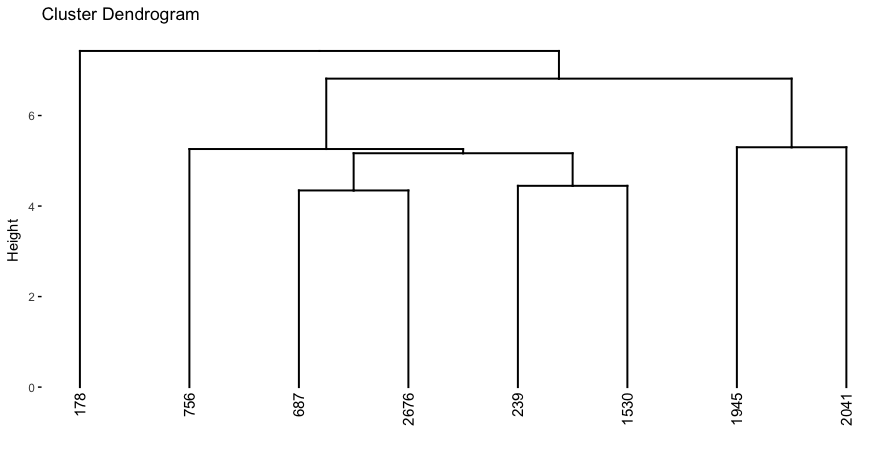
Figure 21.5: A subsection of the dendrogram for illustrative purposes.
However, dendrograms are often misinterpreted. Conclusions about the proximity of two observations should not be implied by their relationship on the horizontal axis nor by the vertical connections. Rather, the height of the branch between an observation and the clusters of observations below them indicate the distance between the observation and that cluster it is joined to. For example, consider observation 9 & 2 in Figure 21.6. They appear close on the dendrogram (right) but, in fact, their closeness on the dendrogram imply they are approximately the same distance measure from the cluster that they are fused to (observations 5, 7, & 8). It by no means implies that observation 9 & 2 are close to one another.
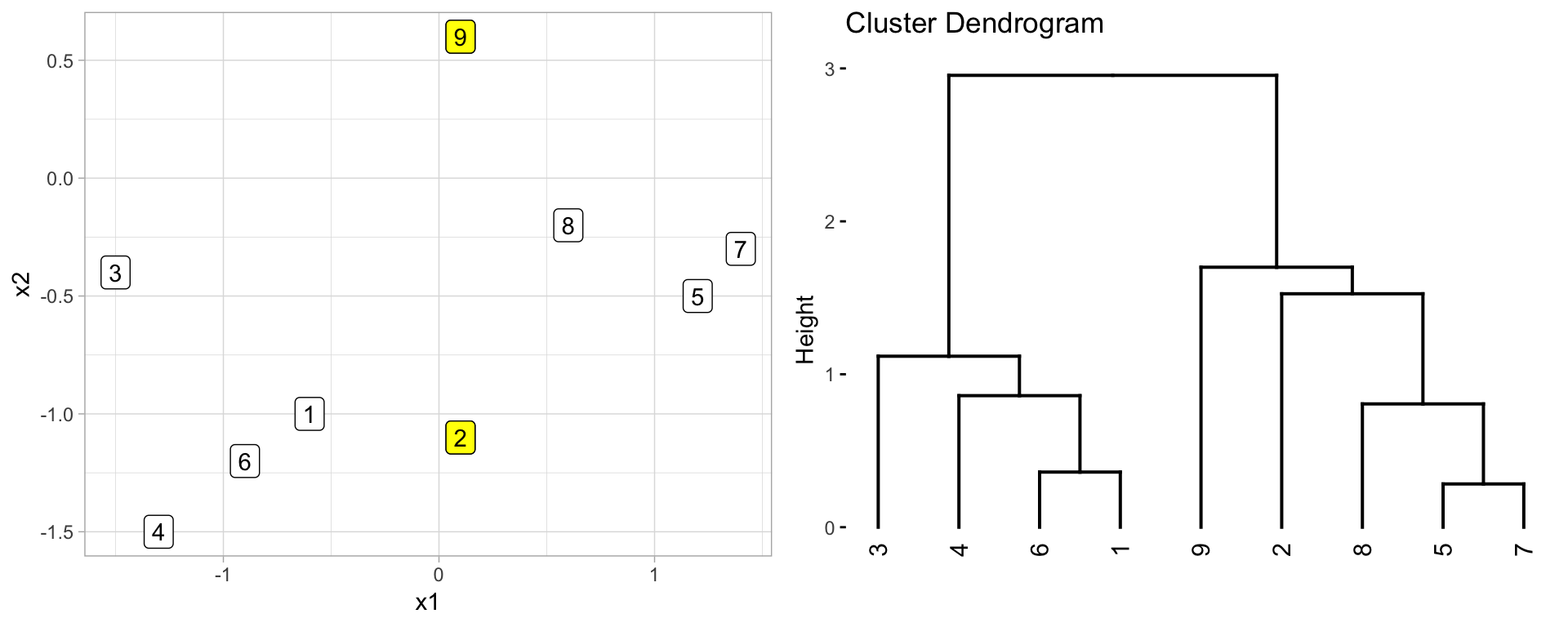
Figure 21.6: Comparison of nine observations measured across two features (left) and the resulting dendrogram created based on hierarchical clustering (right).
In order to identify sub-groups (i.e., clusters), we can cut the dendrogram with cutree(). The height of the cut to the dendrogram controls the number of clusters obtained. It plays the same role as the \(k\) in k-means clustering. Here, we cut our agglomerative hierarchical clustering model into eight clusters. We can see that the concentration of observations are in clusters 1–3.
# Ward's method
hc5 <- hclust(d, method = "ward.D2" )

# Cut tree into 4 groups
sub_grp <- cutree(hc5, k = 8)

# Number of members in each cluster
table(sub_grp)
## sub_grp
##    1    2    3    4    5    6    7    8
## 1363  567  650   36  123  156   24   11
We can plot the entire dendrogram with fviz_dend and highlight the eight clusters with k = 8.
# Plot full dendogram
fviz_dend(
  hc5,
  k = 8,
  horiz = TRUE,
  rect = TRUE,
  rect_fill = TRUE,
  rect_border = "jco",
  k_colors = "jco",
  cex = 0.1
)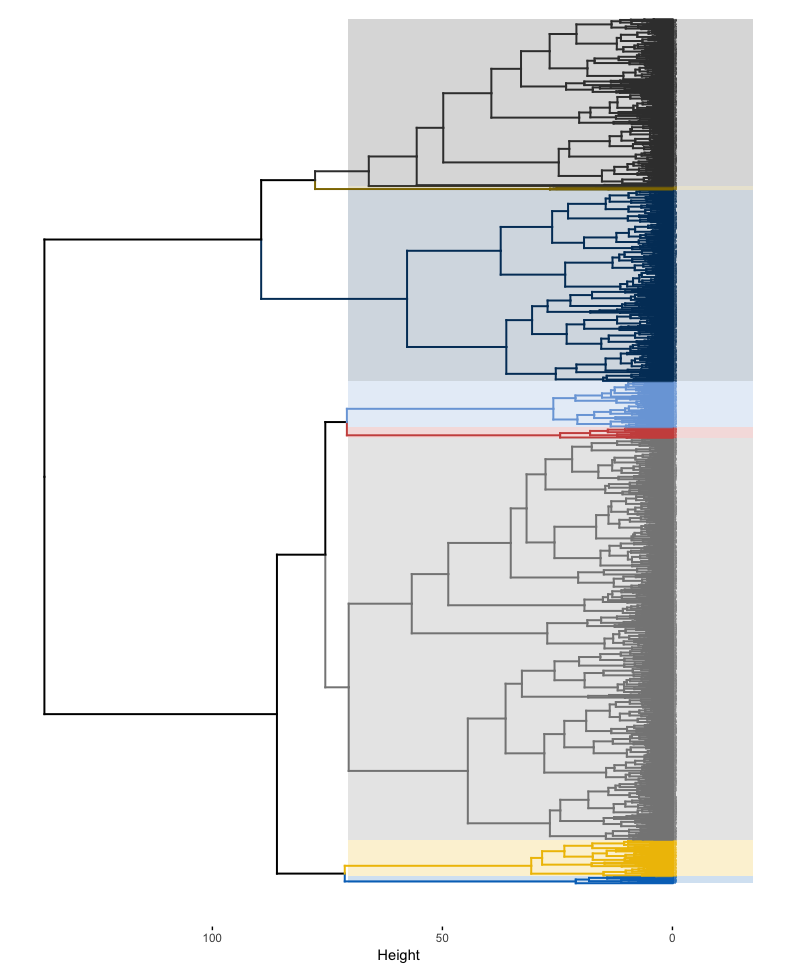
Figure 21.7: The complete dendogram highlighting all 8 clusters.
However, due to the size of the Ames housing data, the dendrogram is not very legible. Consequently, we may want to zoom into one particular region or cluster. This allows us to see which observations are most similar within a particular group.
There is no easy way to get the exact height required to capture all eight clusters. This is largely trial and error by using different heights until the output of dend_cuts() matches the cluster totals identified previously.
dend_plot <- fviz_dend(hc5)                # create full dendogram
dend_data <- attr(dend_plot, "dendrogram") # extract plot info
dend_cuts <- cut(dend_data, h = 70.5)      # cut the dendogram at
                                           # designated height
# Create sub dendrogram plots
p1 <- fviz_dend(dend_cuts$lower[[1]])
p2 <- fviz_dend(dend_cuts$lower[[1]], type = 'circular')

# Side by side plots
gridExtra::grid.arrange(p1, p2, nrow = 1)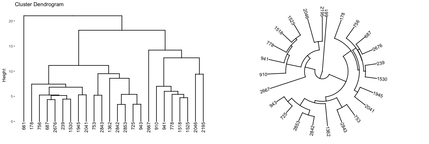
Figure 21.8: A subsection of the dendrogram highlighting cluster 7.
21.6 Final thoughts
Hierarchical clustering may have some benefits over k-means such as not having to pre-specify the number of clusters and the fact that it can produce a nice hierarchical illustration of the clusters (that’s useful for smaller data sets). However, from a practical perspective, hierarchical clustering analysis still involves a number of decisions that can have large impacts on the interpretation of the results. First, like k-means, you still need to make a decision on the dissimilarity measure to use.
Second, you need to make a decision on the linkage method. Each linkage method has different systematic tendencies (or biases) in the way it groups observations and can result in significantly different results. For example, the centroid method has a bias toward producing irregularly shaped clusters. Ward’s method tends to produce clusters with roughly the same number of observations and the solutions it provides tend to be heavily distorted by outliers. Given such tendencies, there should be a match between the algorithm selected and the underlying structure of the data (e.g., sample size, distribution of observations, and what types of variables are included-nominal, ordinal, ratio, or interval). For example, the centroid method should primarily be used when (a) data are measured with interval or ratio scales and (b) clusters are expected to be very dissimilar from each other. Likewise, Ward’s method is best suited for analyses where (a) the number of observations in each cluster is expected to be approximately equal and (b) there are no outliers (Ketchen and Shook 1996).
Third, although we do not need to pre-specify the number of clusters, we often still need to decide where to cut the dendrogram in order to obtain the final clusters to use. So the onus is still on us to decide the number of clusters, albeit in the end. In Chapter 22 we discuss a method that relieves us of this decision.
References
Hair, Joseph F. 2006. Multivariate Data Analysis. Pearson Education India.
Kaufman, Leonard, and Peter J Rousseeuw. 2009. Finding Groups in Data: An Introduction to Cluster Analysis. Vol. 344. John Wiley & Sons.
Ketchen, David J, and Christopher L Shook. 1996. “The Application of Cluster Analysis in Strategic Management Research: An Analysis and Critique.” Strategic Management Journal 17 (6). Wiley Online Library: 441–58.
Ma, Yi, Harm Derksen, Wei Hong, and John Wright. 2007. “Segmentation of Multivariate Mixed Data via Lossy Data Coding and Compression.” IEEE Transactions on Pattern Analysis and Machine Intelligence 29 (9). IEEE: 1546–62.
Zhang, Wei, Deli Zhao, and Xiaogang Wang. 2013. “Agglomerative Clustering via Maximum Incremental Path Integral.” Pattern Recognition 46 (11). Elsevier: 3056–65.
Zhao, Deli, and Xiaoou Tang. 2009. “Cyclizing Clusters via Zeta Function of a Graph.” In Advances in Neural Information Processing Systems, 1953–60.