Chapter 5 Logistic Regression
Linear regression is used to approximate the (linear) relationship between a continuous response variable and a set of predictor variables. However, when the response variable is binary (i.e., Yes/No), linear regression is not appropriate. Fortunately, analysts can turn to an analogous method, logistic regression, which is similar to linear regression in many ways. This chapter explores the use of logistic regression for binary response variables. Logistic regression can be expanded for multinomial problems (see Faraway (2016a) for discussion of multinomial logistic regression in R); however, that goes beyond our intent here.
5.1 Prerequisites
For this section we’ll use the following packages:
# Helper packages
library(dplyr)     # for data wrangling
library(ggplot2)   # for awesome plotting
library(rsample)   # for data splitting

# Modeling packages
library(caret)     # for logistic regression modeling

# Model interpretability packages
library(vip)       # variable importance
To illustrate logistic regression concepts we’ll use the employee attrition data, where our intent is to predict the Attrition response variable (coded as "Yes"/"No"). As in the previous chapter, we’ll set aside 30% of our data as a test set to assess our generalizability error.
df <- attrition %>% mutate_if(is.ordered, factor, ordered = FALSE)

# Create training (70%) and test (30%) sets for the
# rsample::attrition data.
set.seed(123)  # for reproducibility
churn_split <- initial_split(df, prop = .7, strata = "Attrition")
churn_train <- training(churn_split)
churn_test  <- testing(churn_split)
5.2 Why logistic regression
To provide a clear motivation for logistic regression, assume we have credit card default data for customers and we want to understand if the current credit card balance of a customer is an indicator of whether or not they’ll default on their credit card. To classify a customer as a high- vs. low-risk defaulter based on their balance we could use linear regression; however, the left plot in Figure 5.1 illustrates how linear regression would predict the probability of defaulting. Unfortunately, for balances close to zero we predict a negative probability of defaulting; if we were to predict for very large balances, we would get values bigger than 1. These predictions are not sensible, since of course the true probability of defaulting, regardless of credit card balance, must fall between 0 and 1. These inconsistencies only increase as our data become more imbalanced and the number of outliers increase. Contrast this with the logistic regression line (right plot) that is nonlinear (sigmoidal-shaped).
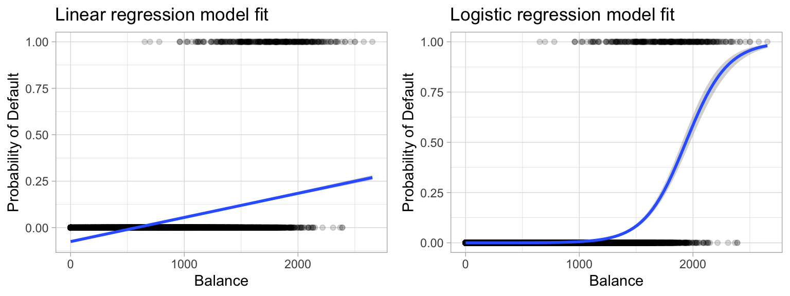
Figure 5.1: Comparing the predicted probabilities of linear regression (left) to logistic regression (right). Predicted probabilities using linear regression results in flawed logic whereas predicted values from logistic regression will always lie between 0 and 1.
To avoid the inadequacies of the linear model fit on a binary response, we must model the probability of our response using a function that gives outputs between 0 and 1 for all values of \(X\). Many functions meet this description. In logistic regression, we use the logistic function, which is defined in Equation (5.1) and produces the S-shaped curve in the right plot above.
\[\begin{equation} \tag{5.1} p\left(X\right) = \frac{e^{\beta_0 + \beta_1X}}{1 + e^{\beta_0 + \beta_1X}} \end{equation}\]
The \(\beta_i\) parameters represent the coefficients as in linear regression and \(p\left(X\right)\) may be interpreted as the probability that the positive class (default in the above example) is present. The minimum for \(p\left(x\right)\) is obtained at \(\lim_{a \rightarrow -\infty} \left[ \frac{e^a}{1+e^a} \right] = 0\), and the maximum for \(p\left(x\right)\) is obtained at \(\lim_{a \rightarrow \infty} \left[ \frac{e^a}{1+e^a} \right] = 1\) which restricts the output probabilities to 0–1. Rearranging Equation (5.1) yields the logit transformation (which is where logistic regression gets its name):
\[\begin{equation} \tag{5.2} g\left(X\right) = \ln \left[ \frac{p\left(X\right)}{1 - p\left(X\right)} \right] = \beta_0 + \beta_1 X \end{equation}\]
Applying a logit transformation to \(p\left(X\right)\) results in a linear equation similar to the mean response in a simple linear regression model. Using the logit transformation also results in an intuitive interpretation for the magnitude of \(\beta_1\): the odds (e.g., of defaulting) increase multiplicatively by \(\exp\left(\beta_1\right)\) for every one-unit increase in \(X\). A similar interpretation exists if \(X\) is categorical; see Agresti (2003), Chapter 5, for details.
5.3 Simple logistic regression
We will fit two logistic regression models in order to predict the probability of an employee attriting. The first predicts the probability of attrition based on their monthly income (MonthlyIncome) and the second is based on whether or not the employee works overtime (OverTime). The glm() function fits generalized linear models, a class of models that includes both logistic regression and simple linear regression as special cases. The syntax of the glm() function is similar to that of lm(), except that we must pass the argument family = "binomial" in order to tell R to run a logistic regression rather than some other type of generalized linear model (the default is family = "gaussian", which is equivalent to ordinary linear regression assuming normally distributed errors).
model1 <- glm(Attrition ~ MonthlyIncome, family = "binomial", data = churn_train)
model2 <- glm(Attrition ~ OverTime, family = "binomial", data = churn_train)
In the background glm() uses ML estimation to estimate the unknown model parameters. The basic intuition behind using ML estimation to fit a logistic regression model is as follows: we seek estimates for \(\beta_0\) and \(\beta_1\) such that the predicted probability \(\widehat p\left(X_i\right)\) of attrition for each employee corresponds as closely as possible to the employee’s observed attrition status. In other words, we try to find \(\widehat \beta_0\) and \(\widehat \beta_1\) such that plugging these estimates into the model for \(p\left(X\right)\) (Equation (5.1)) yields a number close to one for all employees who attrited, and a number close to zero for all employees who did not. This intuition can be formalized using a mathematical equation called a likelihood function:
\[\begin{equation} \tag{5.3} \ell\left(\beta_0, \beta_1\right) = \prod_{i:y_i=1}p\left(X_i\right) \prod_{i':y_i'=0}\left[1-p\left(x_i'\right)\right] \end{equation}\]
The estimates \(\widehat \beta_0\) and \(\widehat \beta_1\) are chosen to maximize this likelihood function. What results is the predicted probability of attrition. Figure 5.2 illustrates the predicted probabilities for the two models.
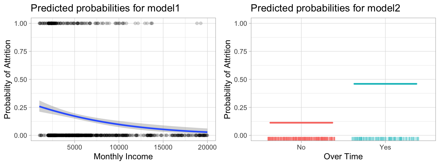
Figure 5.2: Predicted probablilities of employee attrition based on monthly income (left) and overtime (right). As monthly income increases, model1 predicts a decreased probability of attrition and if employees work overtime model2 predicts an increased probability.
The table below shows the coefficient estimates and related information that result from fitting a logistic regression model in order to predict the probability of Attrition = Yes for our two models. Bear in mind that the coefficient estimates from logistic regression characterize the relationship between the predictor and response variable on a log-odds (i.e., logit) scale.
For model1, the estimated coefficient for MonthlyIncome is \(\widehat \beta_1 =\) -0.000130, which is negative, indicating that an increase in MonthlyIncome is associated with a decrease in the probability of attrition. Similarly, for model2, employees who work OverTime are associated with an increased probability of attrition compared to those that do not work OverTime.
tidy(model1)
## # A tibble: 2 x 5
##   term           estimate std.error statistic       p.value
##   <chr>             <dbl>     <dbl>     <dbl>         <dbl>
## 1 (Intercept)   -0.924    0.155         -5.96 0.00000000259
## 2 MonthlyIncome -0.000130 0.0000264     -4.93 0.000000836
tidy(model2)
## # A tibble: 2 x 5
##   term        estimate std.error statistic  p.value
##   <chr>          <dbl>     <dbl>     <dbl>    <dbl>
## 1 (Intercept)    -2.18     0.122    -17.9  6.76e-72
## 2 OverTimeYes     1.41     0.176      8.00 1.20e-15
As discussed earlier, it is easier to interpret the coefficients using an \(\exp()\) transformation:
exp(coef(model1))
##   (Intercept) MonthlyIncome
##     0.3970771     0.9998697
exp(coef(model2))
## (Intercept) OverTimeYes
##   0.1126126   4.0812121
Thus, the odds of an employee attriting in model1 increase multiplicatively by 0.9999 for every one dollar increase in MonthlyIncome, whereas the odds of attriting in model2 increase multiplicatively by 4.0812 for employees that work OverTime compared to those that do not.
Many aspects of the logistic regression output are similar to those discussed for linear regression. For example, we can use the estimated standard errors to get confidence intervals as we did for linear regression in Chapter 4:
confint(model1)  # for odds, you can use `exp(confint(model1))`
##                       2.5 %        97.5 %
## (Intercept)   -1.2267754960 -6.180062e-01
## MonthlyIncome -0.0001849796 -8.107634e-05
confint(model2)
##                 2.5 %    97.5 %
## (Intercept) -2.430458 -1.952330
## OverTimeYes  1.063246  1.752879
5.4 Multiple logistic regression
We can also extend our model as seen in Equation 1 so that we can predict a binary response using multiple predictors:
\[\begin{equation} \tag{5.4} p\left(X\right) = \frac{e^{\beta_0 + \beta_1 X + \cdots + \beta_p X_p }}{1 + e^{\beta_0 + \beta_1 X + \cdots + \beta_p X_p}} \end{equation}\]
Let’s go ahead and fit a model that predicts the probability of Attrition based on the MonthlyIncome and OverTime. Our results show that both features are statistically significant (at the 0.05 level) and Figure 5.3 illustrates common trends between MonthlyIncome and Attrition; however, working OverTime tends to nearly double the probability of attrition.
model3 <- glm(
  Attrition ~ MonthlyIncome + OverTime,
  family = "binomial",
  data = churn_train
  )

tidy(model3)
## # A tibble: 3 x 5
##   term           estimate std.error statistic  p.value
##   <chr>             <dbl>     <dbl>     <dbl>    <dbl>
## 1 (Intercept)   -1.43     0.176         -8.11 5.25e-16
## 2 MonthlyIncome -0.000139 0.0000270     -5.15 2.62e- 7
## 3 OverTimeYes    1.47     0.180          8.16 3.43e-16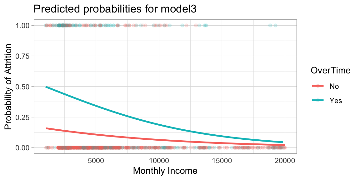
Figure 5.3: Predicted probability of attrition based on monthly income and whether or not employees work overtime.
5.5 Assessing model accuracy
With a basic understanding of logistic regression under our belt, similar to linear regression our concern now shifts to how well do our models predict. As in the last chapter, we’ll use caret::train() and fit three 10-fold cross validated logistic regression models. Extracting the accuracy measures (in this case, classification accuracy), we see that both cv_model1 and cv_model2 had an average accuracy of 83.88%. However, cv_model3 which used all predictor variables in our data achieved an average accuracy rate of 87.58%.
set.seed(123)
cv_model1 <- train(
  Attrition ~ MonthlyIncome,
  data = churn_train,
  method = "glm",
  family = "binomial",
  trControl = trainControl(method = "cv", number = 10)
)

set.seed(123)
cv_model2 <- train(
  Attrition ~ MonthlyIncome + OverTime,
  data = churn_train,
  method = "glm",
  family = "binomial",
  trControl = trainControl(method = "cv", number = 10)
)

set.seed(123)
cv_model3 <- train(
  Attrition ~ .,
  data = churn_train,
  method = "glm",
  family = "binomial",
  trControl = trainControl(method = "cv", number = 10)
)

# extract out of sample performance measures
summary(
  resamples(
    list(
      model1 = cv_model1,
      model2 = cv_model2,
      model3 = cv_model3
    )
  )
)$statistics$Accuracy
##             Min.   1st Qu.    Median      Mean   3rd Qu.      Max. NA's
## model1 0.8349515 0.8349515 0.8365385 0.8388478 0.8431373 0.8446602    0
## model2 0.8349515 0.8349515 0.8365385 0.8388478 0.8431373 0.8446602    0
## model3 0.8365385 0.8495146 0.8792476 0.8757893 0.8907767 0.9313725    0
We can get a better understanding of our model’s performance by assessing the confusion matrix (see Section 2.6). We can use caret::confusionMatrix() to compute a confusion matrix. We need to supply our model’s predicted class and the actuals from our training data. The confusion matrix provides a wealth of information. Particularly, we can see that although we do well predicting cases of non-attrition (note the high specificity), our model does particularly poor predicting actual cases of attrition (note the low sensitivity).
By default the predict() function predicts the response class for a caret model; however, you can change the type argument to predict the probabilities (see ?caret::predict.train).
# predict class
pred_class <- predict(cv_model3, churn_train)

# create confusion matrix
confusionMatrix(
  data = relevel(pred_class, ref = "Yes"),
  reference = relevel(churn_train$Attrition, ref = "Yes")
)
## Confusion Matrix and Statistics
##
##           Reference
## Prediction Yes  No
##        Yes  93  25
##        No   73 839
##
##                Accuracy : 0.9049
##                  95% CI : (0.8853, 0.9221)
##     No Information Rate : 0.8388
##     P-Value [Acc > NIR] : 5.360e-10
##
##                   Kappa : 0.6016
##
##  Mcnemar's Test P-Value : 2.057e-06
##
##             Sensitivity : 0.56024
##             Specificity : 0.97106
##          Pos Pred Value : 0.78814
##          Neg Pred Value : 0.91996
##              Prevalence : 0.16117
##          Detection Rate : 0.09029
##    Detection Prevalence : 0.11456
##       Balanced Accuracy : 0.76565
##
##        'Positive' Class : Yes
##
One thing to point out, in the confusion matrix above you will note the metric No Information Rate: 0.839. This represents the ratio of non-attrition vs. attrition in our training data (table(churn_train$Attrition) %>% prop.table()). Consequently, if we simply predicted "No" for every employee we would still get an accuracy rate of 83.9%. Therefore, our goal is to maximize our accuracy rate over and above this no information baseline while also trying to balance sensitivity and specificity. To that end, we plot the ROC curve (section 2.6) which is displayed in Figure 5.4. If we compare our simple model (cv_model1) to our full model (cv_model3), we see the lift achieved with the more accurate model.
library(ROCR)

# Compute predicted probabilities
m1_prob <- predict(cv_model1, churn_train, type = "prob")$Yes
m3_prob <- predict(cv_model3, churn_train, type = "prob")$Yes

# Compute AUC metrics for cv_model1 and cv_model3
perf1 <- prediction(m1_prob, churn_train$Attrition) %>%
  performance(measure = "tpr", x.measure = "fpr")
perf2 <- prediction(m3_prob, churn_train$Attrition) %>%
  performance(measure = "tpr", x.measure = "fpr")

# Plot ROC curves for cv_model1 and cv_model3
plot(perf1, col = "black", lty = 2)
plot(perf2, add = TRUE, col = "blue")
legend(0.8, 0.2, legend = c("cv_model1", "cv_model3"),
       col = c("black", "blue"), lty = 2:1, cex = 0.6)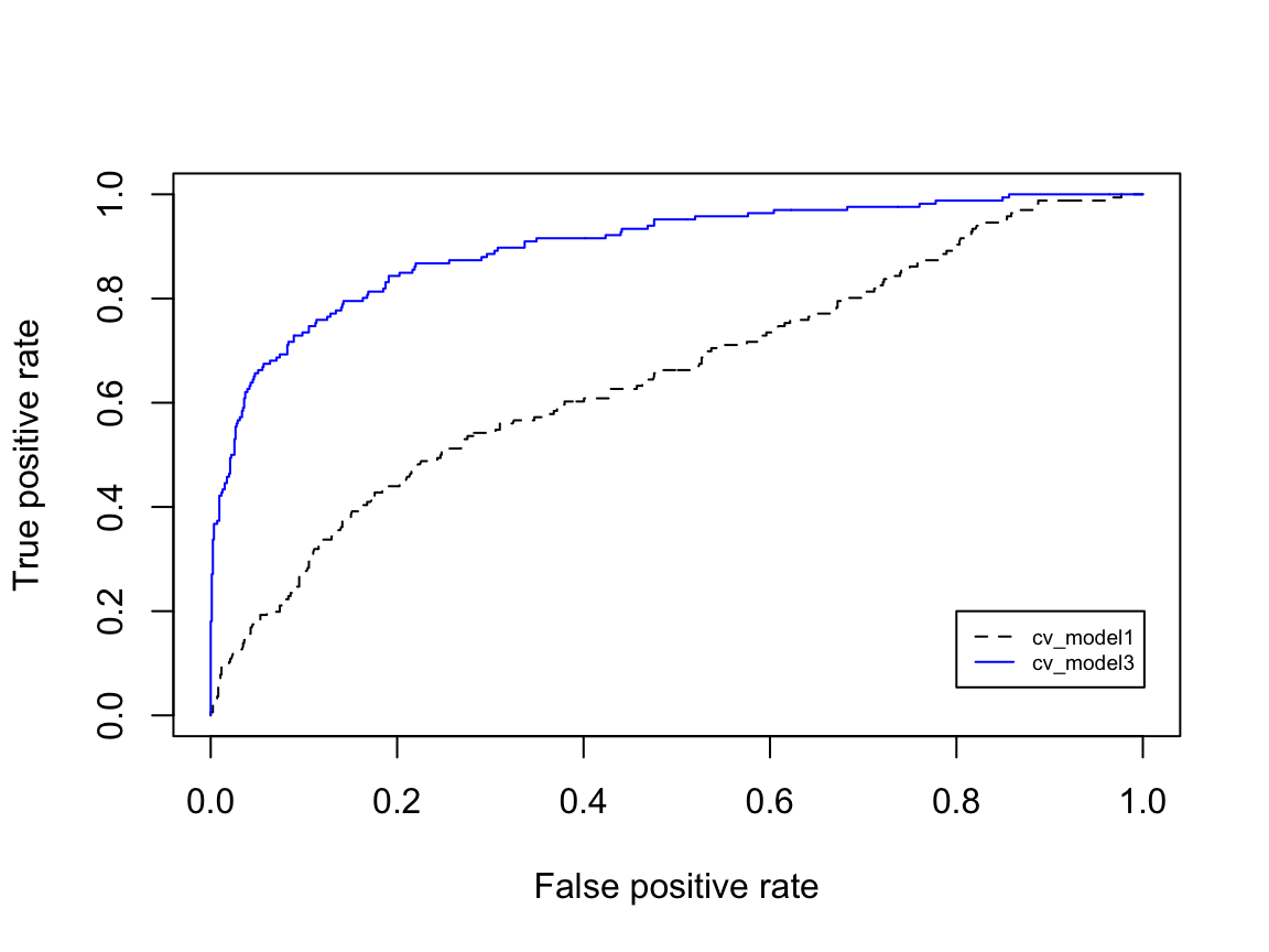
Figure 5.4: ROC curve for cross-validated models 1 and 3. The increase in the AUC represents the ‘lift’ that we achieve with model 3.
Similar to linear regression, we can perform a PLS logistic regression to assess if reducing the dimension of our numeric predictors helps to improve accuracy. There are 16 numeric features in our data set so the following code performs a 10-fold cross-validated PLS model while tuning the number of principal components to use from 1–16. The optimal model uses 14 principal components, which is not reducing the dimension by much. However, the mean accuracy of 0.876 is no better than the average CV accuracy of cv_model3 (0.876).
# Perform 10-fold CV on a PLS model tuning the number of PCs to
# use as predictors
set.seed(123)
cv_model_pls <- train(
  Attrition ~ .,
  data = churn_train,
  method = "pls",
  family = "binomial",
  trControl = trainControl(method = "cv", number = 10),
  preProcess = c("zv", "center", "scale"),
  tuneLength = 16
)

# Model with lowest RMSE
cv_model_pls$bestTune
##    ncomp
## 14    14

# results for model with lowest loss
cv_model_pls$results %>%
  dplyr::filter(ncomp == pull(cv_model_pls$bestTune))
##   ncomp  Accuracy     Kappa AccuracySD   KappaSD
## 1    14 0.8757518 0.3766944 0.01919777 0.1142592

# Plot cross-validated RMSE
ggplot(cv_model_pls)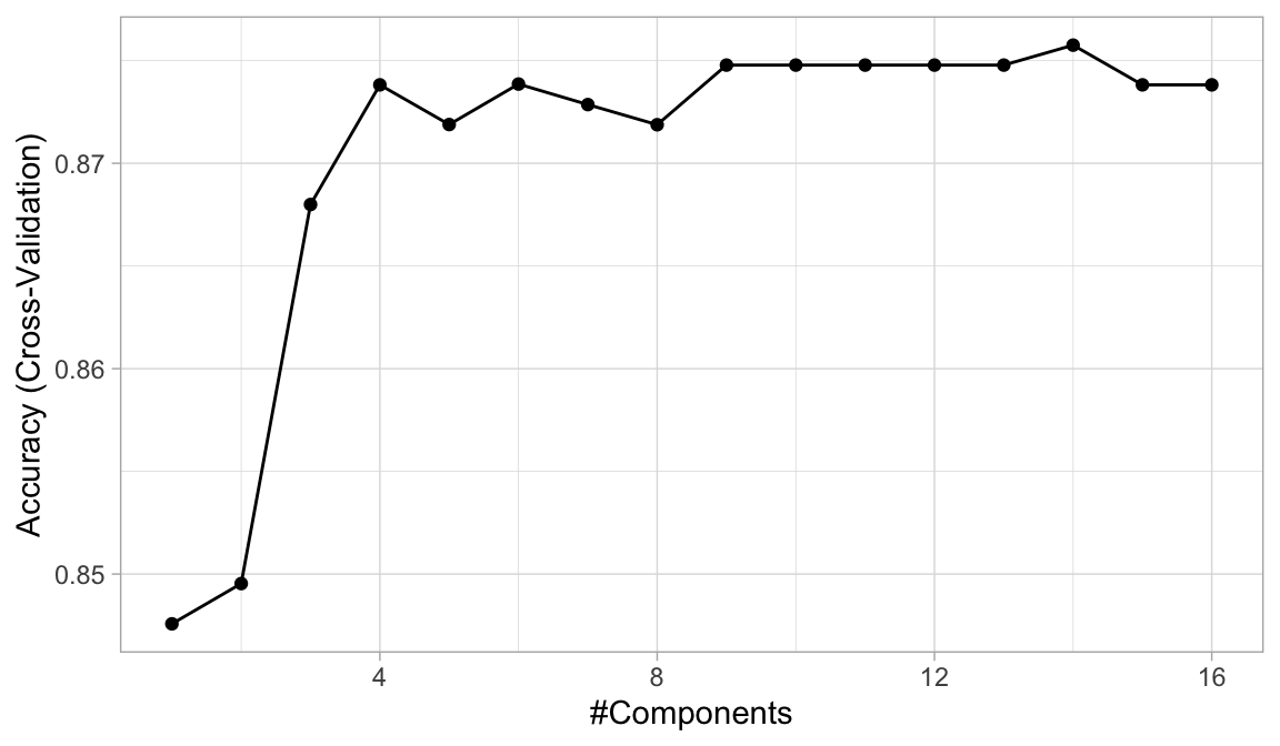
Figure 5.5: The 10-fold cross-validation RMSE obtained using PLS with 1–16 principal components.
5.6 Model concerns
As with linear models, it is important to check the adequacy of the logistic regression model (in fact, this should be done for all parametric models). This was discussed for linear models in Section 4.5 where the residuals played an important role. Although not as common, residual analysis and diagnostics are equally important to generalized linear models. The problem is that there is no obvious way to define what a residual is for more general models. For instance, how might we define a residual in logistic regression when the outcome is either 0 or 1? Nonetheless attempts have been made and a number of useful diagnostics can be constructed based on the idea of a pseudo residual; see, for example, Harrell (2015), Section 10.4.
More recently, Liu and Zhang (2018) introduced the concept of surrogate residuals that allows for residual-based diagnostic procedures and plots not unlike those in traditional linear regression (e.g., checking for outliers and misspecified link functions). For an overview with examples in R using the sure package, see Brandon M. Greenwell et al. (2018).
5.7 Feature interpretation
Similar to linear regression, once our preferred logistic regression model is identified, we need to interpret how the features are influencing the results. As with normal linear regression models, variable importance for logistic regression models can be computed using the absolute value of the \(z\)-statistic for each coefficient (albeit with the same issues previously discussed). Using vip::vip() we can extract our top 20 influential variables. Figure 5.6 illustrates that OverTime is the most influential followed by JobSatisfaction, and EnvironmentSatisfaction.
vip(cv_model3, num_features = 20)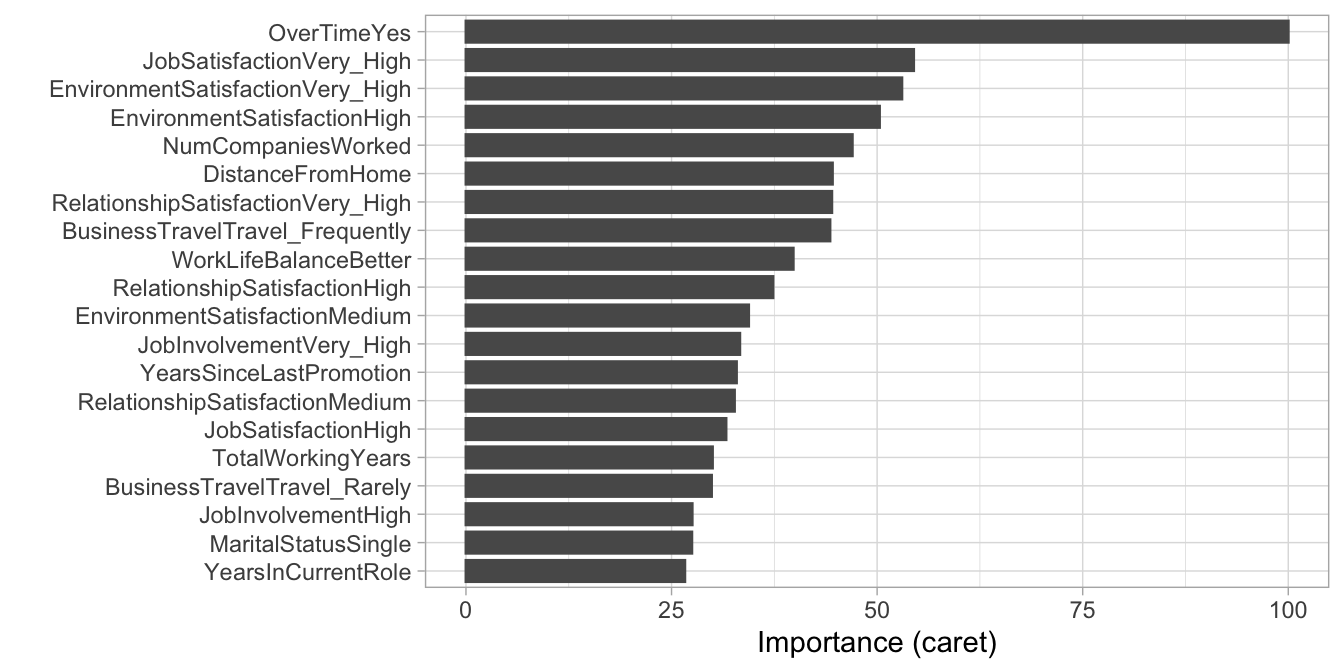
Figure 5.6: Top 20 most important variables for the PLS model.
Similar to linear regression, logistic regression assumes a monotonic linear relationship. However, the linear relationship occurs on the logit scale; on the probability scale, the relationship will be nonlinear. This is illustrated by the PDP in Figure 5.7 which illustrates the functional relationship between the predicted probability of attrition and the number of companies an employee has worked for (NumCompaniesWorked) while taking into account the average effect of all the other predictors in the model. Employees who’ve experienced more employment changes tend to have a high probability of making another change in the future.
Furthermore, the PDPs for the top three categorical predictors (OverTime, JobSatisfaction, and EnvironmentSatisfaction) illustrate the change in predicted probability of attrition based on the employee’s status for each predictor.
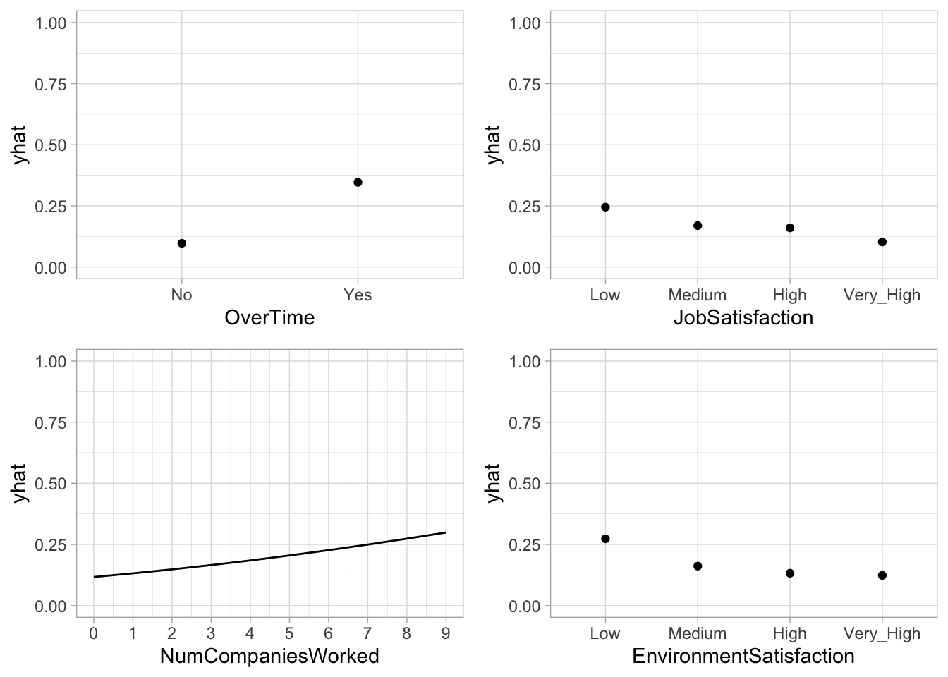
Figure 5.7: Partial dependence plots for the first four most important variables. We can see how the predicted probability of attrition changes for each value of the influential predictors.
5.8 Final thoughts
Logistic regression provides an alternative to linear regression for binary classification problems. However, similar to linear regression, logistic regression suffers from the many assumptions involved in the algorithm (i.e. linear relationship of the coefficient, multicollinearity). Moreover, often we have more than two classes to predict which is commonly referred to as multinomial classification. Although multinomial extensions of logistic regression exist, the assumptions made only increase and, often, the stability of the coefficient estimates (and therefore the accuracy) decrease. Future chapters will discuss more advanced algorithms that provide a more natural and trustworthy approach to binary and multinomial classification prediction.
References
Agresti, Alan. 2003. Categorical Data Analysis. Wiley Series in Probability and Statistics. Wiley.
Faraway, Julian J. 2016a. Extending the Linear Model with R: Generalized Linear, Mixed Effects and Nonparametric Regression Models. Vol. 124. CRC press.
Greenwell, Brandon M., Andrew J. McCarthy, Bradley C. Boehmke, and Dungang Lui. 2018. “Residuals and Diagnostics for Binary and Ordinal Regression Models: An Introduction to the Sure Package.” The R Journal 10 (1): 1–14. https://journal.r-project.org/archive/2018/RJ-2018-004/index.html.
Harrell, Frank E. 2015. Regression Modeling Strategies: With Applications to Linear Models, Logistic and Ordinal Regression, and Survival Analysis. Springer Series in Statistics. Springer International Publishing. https://books.google.com/books?id=94RgCgAAQBAJ.
Liu, Dungang, and Heping Zhang. 2018. “Residuals and Diagnostics for Ordinal Regression Models: A Surrogate Approach.” Journal of the American Statistical Association 113 (522). Taylor & Francis: 845–54. https://doi.org/10.1080/01621459.2017.1292915.
Russolillo, Giorgio, and Carlo Natale Lauro. 2011. “A Proposal for Handling Categorical Predictors in Pls Regression Framework.” In Classification and Multivariate Analysis for Complex Data Structures, 343–50. Springer.